Introduction

Welcome to AP Calculus AB/BC Topic 4.6 - Approximating Values of a Function Using Local Linearity and Linearization. In today's lesson, we are going to talk about tangent lines, and how these tangent lines can give us an approximation of a function's value. This is a fairly straight-forward topic, so with enough practice problems, you should master it quickly.

Tangent Line Review

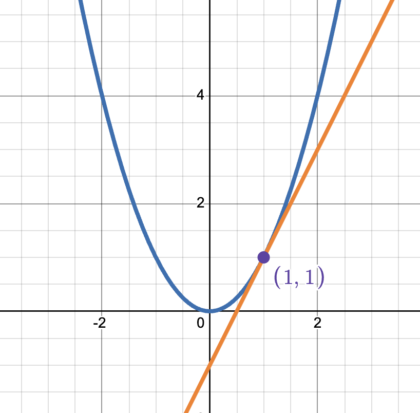
Recall that a tangent line is a straight linear line that touches the curve it is tangent to at a single point without crossing it locally. The tangent line's slope matches the exact slope of the curve at the precise point it touches.

The image below shows a tangent line to the graph of $y=x^2$ at $x=1$. Notice how it touches the graph of $y=x^2$ at one point and matches the exact slope of $y=x^2$ at $x=1$.

Using Tangent Lines to Approximate Values

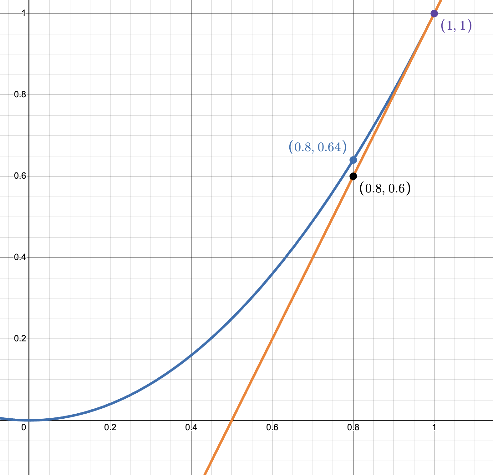
The tangent line of the function $f(x)$ at $x=a$ can give you an approximate value for $f(x)$.

Take a look at the image below. The blue graph is $f(x)=x^2$, and the orange graph is the tangent line of $f(x)$ at $x=1$. We will talk more about how to get the equation of the tangent line later. For now, just focus on the concept visually. In the image below, you can see that we can estimate the value of $f(0.8)$ by using the tangent line of the function $y=x^2$. The true value of $f(0.8)$ is $0.64$, but our approximation of $f(0.8)$ was $0.60$, only $0.04$ off. If we were to try and approximate values even closer to $x=1$, our approximation error would be less. If we were to try and approximate values even farther from $x=1$, our approximation error would be more.

Concave Up vs Concave Down

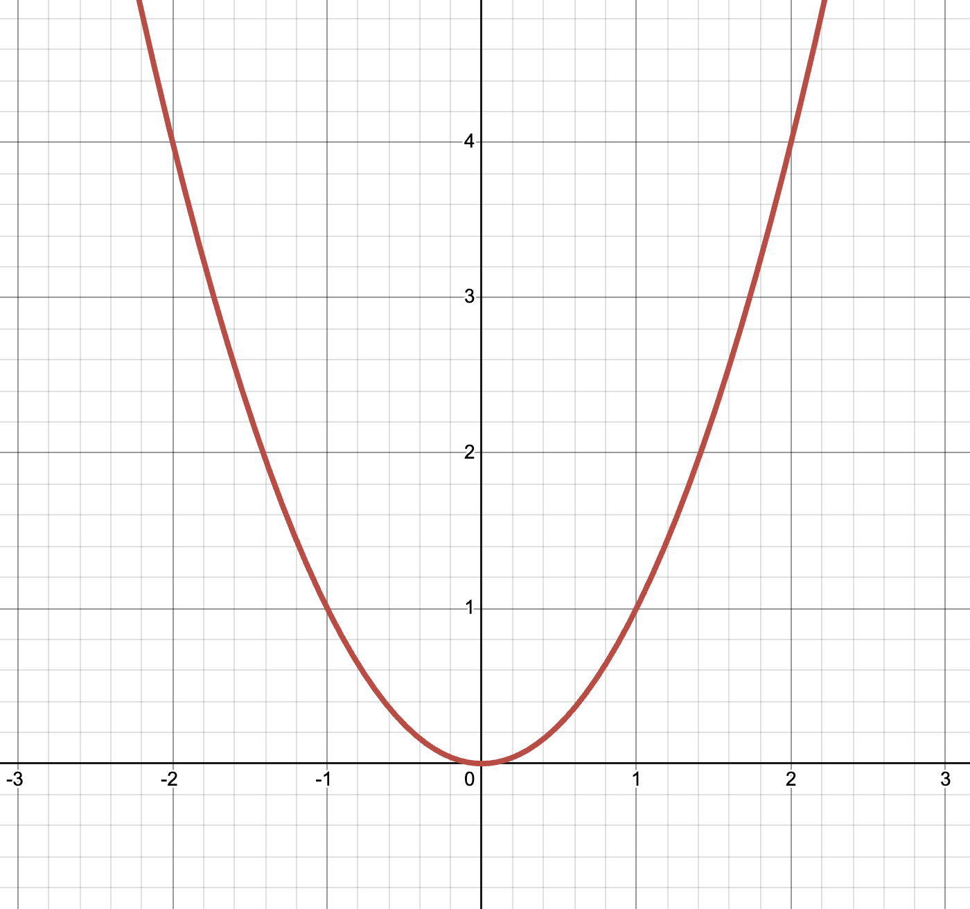
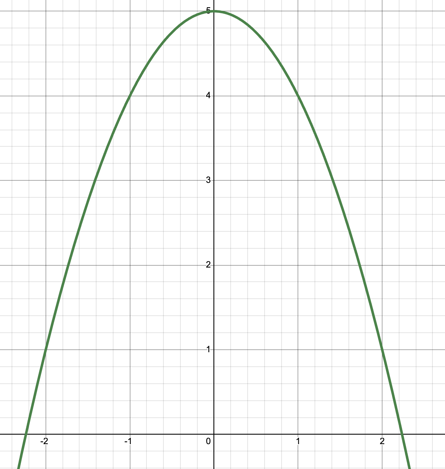
The concavity of a function can tell us whether our tangent line approximations are an overestimate or underestimate. For now, you just need to be able to tell if a function is concave up or concave down based on the graph. Otherwise, you will be told if it is concave up or concave down. In later units, we will be able to determine concavity mathematically. 

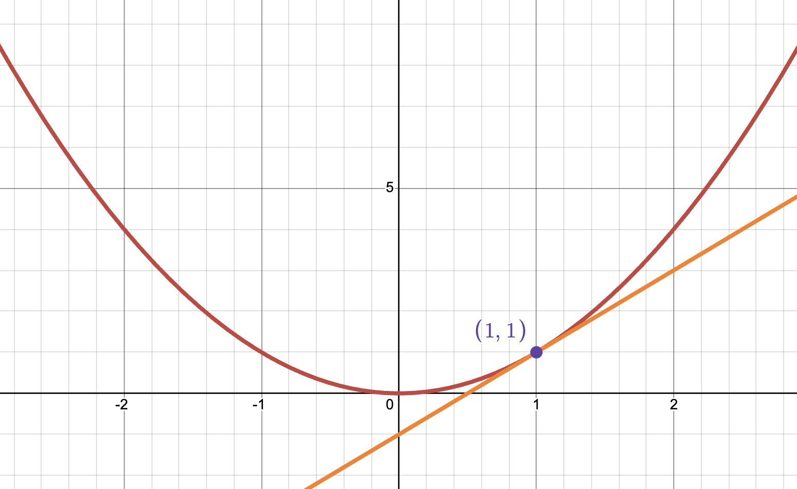
The red graph below is an example of a concave up graph, it looks like a U.

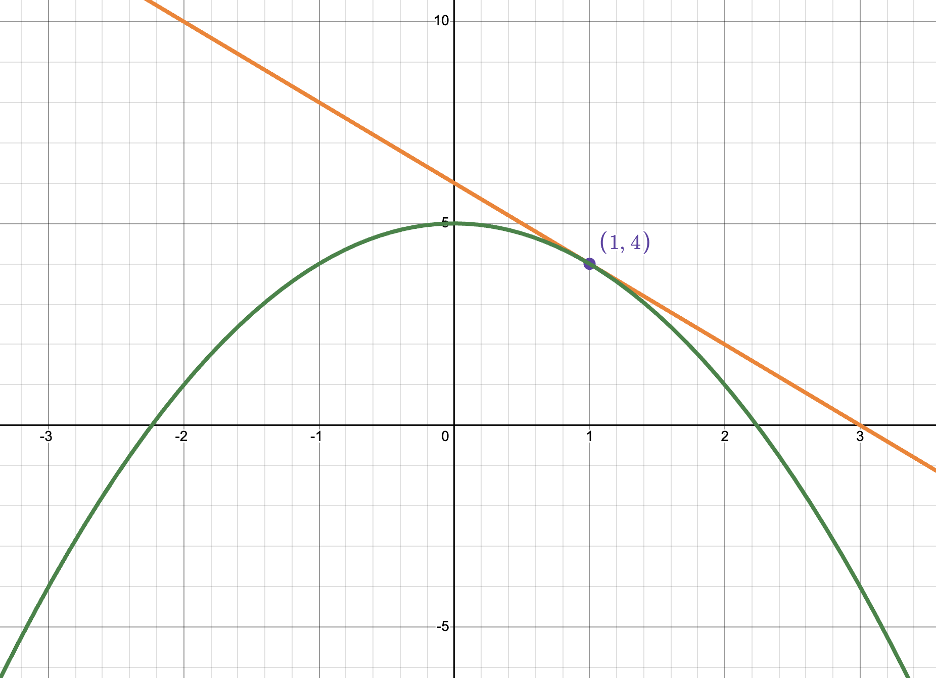
The green graph below is an example of a concave down graph, it looks like a frowny face.

Concavity and Tangent Line Approximations

The most important thing to realize, is that:

1. If a tangent line is used to approximate values for a concave up function, then the approximation is an underestimate.

2. If a tangent line is used to approximate values of a concave down function, then the approximation is an overestimate.

This makes sense visually, because for a concave up function, our tangent line lies below the curve. And for a concave down function, our tangent line lies above the curve.

Take a look at the images below and pay attention to whether the tangent lines lie above or below the curve.

Tangent Line Formula

You should already have learned this in Unit 2, but let's review. 

The equation of the line tangent to the function $f(x)$ at $x=a$ is given by:

$y-f(a)=f^{\prime }(a)(x-a)$

We can re-arrange this formula to isolate $y$:

$y=f(a)+f^{\prime }(a)(x-a)$

This version of the tangent line equation is called the local linear approximation function. Most of the time, we rewrite $y$ as $L(x)$:

$L(x)=f(a)+f^{\prime }(a)(x-a)$

Mathematically, they are the same, but we just swapped $y$ out with $L(x)$ to make it more clear that we are using this tangent line to approximate values.

Combining Everything!

Now that we have learned everything we need to know for this section, let's try some practice. I encourage you to try the questions on your own first.

Practice Section