Introduction

Hi, welcome to the third lesson of Unit 4 for AP CSP. This is the final lesson of Unit 4!

The main purpose of this article is to cover the material in the AP CSP CED. 

Sequential Computing

Traditionally, most programs are made with sequential computing. For example, when executing your code for your Performance Task, you may use a coding language that executes functions or lines in order. Basically, sequential computing means that each instruction to a program is processed once at a time. However, because of how inefficient this can get with a high number of steps (instructions), we need to use alternative methods to combat this.

Parallel Computing

Parallel computing is a method in which program parts can be split into multiple parts that can then be run simultaneously across multiple processors. There are many advantages that come with using parallel computing, such as its time, resource, and cost efficiency and its scalability (see 4.1 to review) compared to sequential computing.  For example, if you added 2 new steps inside a program, the single processor of the sequential computing has to go through those two steps. However, if you apply parallel computing, 2 processors could run 1 step each, speeding it up. Now imagine if even more steps were added, parallel computing could help run it much more efficiently. 

Distributed Computing

Distributed computing is a method in which multiple computing devices are used to run the same program. This essentially allows for multiple “people” or processors to be working on the same problem or program, speeding it up. In addition, it reduces the amount of storage required to run the program as the data could be split between multiple devices.

Because of their designs, distributed and parallel computing have the potential to analyze large data sets and process them multiple times faster than sequential computing. 

Computing Efficiency

In order to calculate computing time, let's look at an example. 

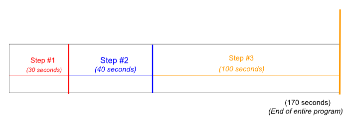
Given an arbitrary program with 3 steps: 

If we were to run this program sequentially, or with each step in order, it would take 170 seconds (40 + 30 + 100).

However, if we had two processors and the steps could be run in parallel, we could run Step 1 and Step 2 on one processor while simultaneously running Step 3 on another processor. This means it would only take 100 seconds for the program to run.  

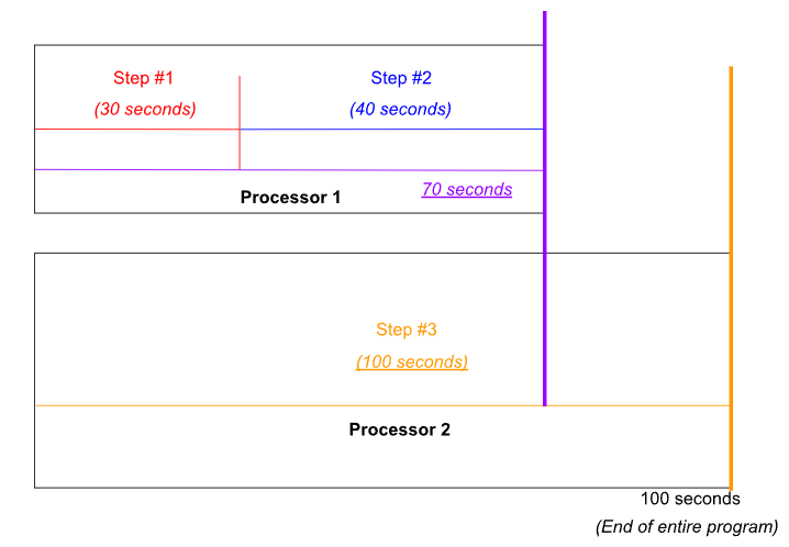
Now let's calculate the speedup of parallel computing. It is the ratio of the time when run in parallel to the time when run sequentially. For this example, we have a speedup of 1.7 meaning that running this program in parallel is 1.7 times faster than running it sequentially.

Limitations

However, parallel computing does have its limitations. Let’s look back at the same question with the three steps.

Now we are given the information that Steps 2 and 3 require the results from Step 1. What does this mean?

Well it means that we cannot run Steps 2 or 3 without first running Step 1. Because of this, Step 1 must first be run sequentially, before splitting Steps 2 and 3 across the two processors. This means that the total time for the program to be run parallel is 140 seconds. 

In essence, parallel computing is limited only by the amount of time taken for steps that must be run sequentially. 

Practice Problems