Introduction

Welcome to the FiveHive article for Unit 1.3 of AP Physics 1! 

In this unit, we will be covering the representation of motion. This will be done through kinematic equations and also kinematic graphs.

As usual, we will only cover what is mentioned on the CED for Unit 1.3. 

Describing Motion

The motion of an object is described through three different components: position, acceleration, and velocity. Using these components, we can describe motion through kinematic equations and graphs for each of the components. 

For constant, or uniform, acceleration, there are three equations that can be used to describe instantaneous linear motion in one dimension:

$vx=v_{xo}+a_{x}t$

$\Delta x=x_o+v_{xo}t+\frac{1}{2}a{t}^2$

$v_x^2=v_o^2+2a(\Delta x)$

These equations are instrumental in describing and predicting an object’s motion. Keep in mind, these three are not the only kinematic equations. However, for our current purposes, they are enough. 

You may have noticed that some of the variables have a subscript of $x$. This does not mean that these equations can only be used in the $x$-direction. In fact, they are often used to predict the vertical motion of projectiles or the motion of an object dropped straight down. Instead, the subscript is there to serve more as a reminder that all the variables have to be components of the same axis. 

Vertical Application of Kinematic Equations

Speaking of multidimensional applications of these equations, let’s familiarize ourselves with how these equations can change for the vertical axis. 

An important change in the representation of these equations is how acceleration is denoted. While horizontal acceleration is often denoted with $a$ or $a_x$, vertical acceleration is $g$. 

This value is known as the acceleration due to gravity. Near the surface of the Earth, the acceleration caused by the force of gravity is constant, downward, and has a value approximately equal to:

$a_g=g\approx 10m/{\mathrm{s}}^2$

This acceleration due to gravity is often what we will use for kinematics applied on the $y$-axis instead of $a_x$. 

BEWARE!!

While we may refer to $a_y=g$ as ‘little g’ colloquially, it is imperative that you do not refer to this value as such on FRQs! ‘Little g’ is to be referred to as, and ONLY as, acceleration due to gravity. 

Representation of Motion With Graphs

Aside from equations, the motion of an object is often represented using motion graphs. These graphs describe the position, velocity, and acceleration of the object separately. 

For instance, let us take into consideration a ball being thrown up and being caught as it comes back down. The motion graphs for this situation can be drawn as such:

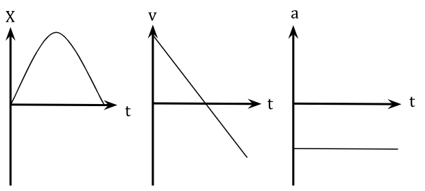
Notice how even though the ball has no horizontal motion, we still label the $y$-axis of the position graph as $x$!

Additionally, upon close inspection of the three graphs in tandem, it would appear that the velocity graph is the rate of change of the position graph, and the acceleration graph is the rate of change of the velocity graph. 

This is no coincidence! In all applications of these graphs, the velocity is always the rate of change of position, and the acceleration is always the rate of change of velocity. You can also work backwards from the acceleration graph by noticing that its area is the change in velocity, and its area is the change in position!

Practice

I have some great news for you: you have made it through unit 1.3 of AP Physics 1! What a great feat! Let’s keep rolling with this momentum (wink, wink!). Now, it is time to put the knowledge you have acquired to the test with some MCQs.