Sampling Distributions for Sample Proportions

Introduction

In Topic 3.1 of AP Statistics, we learned all about estimators and how things like sample proportions can be a good estimate for the population proportion. With this lesson, we continue on our journey of Inferential Statistics by discussing one of the most important concepts of AP Statistics: Sampling distribution. Understanding this topic is even more imperative if one wishes to uncover the rest of AP Statistics.

What is a Sampling Distribution?

A sampling distribution is the probability distribution of a statistic (like $\hat{p}$) across all possible samples of the same size from a population.

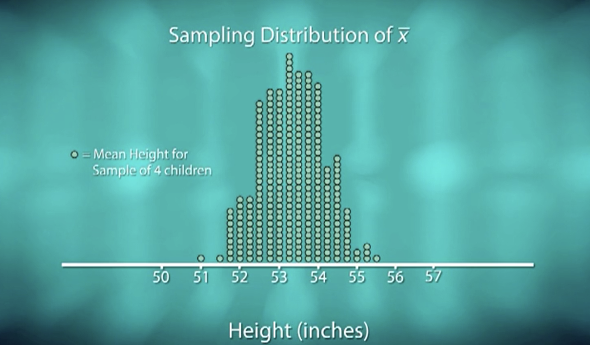
Let’s back up. Think about this: if we were looking for the mean of the heights of ALL 6th graders in one classroom, it would be helpful to look at maybe a few individuals to conduct a sample. Let’s say our sample size will be 4 students. So, we will take 4 students out into the hallway, measure the height of all 4, and then average them into a mean or $\bar{x}$. When we do this, we just created one piece of data for our sampling distribution. Let’s grab another 4 random students, measure them all, then find the mean of this sample. And as we do this, we can get many, many, many means from this one classroom, especially if our sample might contain repeated individuals. Over time, if we do this over and over, and plot them onto a chart, we will get a sampling distribution.

So, a sampling distribution is a distribution of a single statistic (like x-bar) across ALL possible samples of the same sample size from a population.

A Concrete Example

Now, the prior example was for means. This chapter is all about proportions. Let’s think about an example.

If every single person in a graduating high school class bought one share-size bag of M&M’s, and the true proportion of red M&M’s in every single bag was $p=0.30$, this means that for every single person’s bag of M&M’s, for every 10 M&M’s, 3 of them were red. This is what the manufacturer claims.

Now, if I choose to randomly select one student, open their bag, and count how many M&M’s were red, divided by the total number of M&M’s in their bag, it will give us a sample proportion of $\hat{p}$.

So let’s say somebody has 19 red ones out of 50 total M&M’s.

$\hat{p}=\frac{19}{50}=0.38$.

Perhaps we look at another student’s bag:

$\hat{p}=\frac{11}{50}=0.22$.

Perhaps another:

$\hat{p}=\frac{15}{50}=0.30$ 

And we kept going more and more, looking into every single student’s bag and finding the proportion. So here, our sample size is 50, because there are 50 M&M’s.

The sampling distribution shows us the pattern of all these possible $\hat{p}$ values. It tells us which values are common (near 0.30) and which are rare (far from 0.30).

Why This Matters

The sampling distribution allows us to:

Mean of the Sampling Distribution

The mean of the sampling distribution of $\hat{p}$ is denoted ${\mu }_{\hat{p}}$ and equals the population proportion:

${\mu }_{\hat{p}}=p$

This makes intuitive sense and confirms what we learned in Topic 3.1: the sample proportion is an unbiased estimator. On average, across all possible samples, $\hat{p}$ equals $p$.

What This Tells Us

If $p=0.45$, then ${\mu }_{\hat{p}}=0.45$. This means:

Standard Deviation of the Sampling Distribution

While the mean tells us where the sampling distribution is centered, the standard deviation tells us how spread out it is. The standard deviation of the sampling distribution of $\hat{p}$ is:

${\sigma }_{\hat{p}}=\sqrt{\frac{p(1-p)}{n}}$

This formula is sometimes called the standard error of $\hat{p}$, though technically "standard error" refers to when we estimate this value using $\hat{p}$ instead of $p$.

Understanding the Formula

Let’s talk about the spread of the sampling distribution, the same way we talked about spread when describing distributions.

Example Calculation

If $p=0.35$ and $n=200$, calculate ${\sigma }_{\hat{p}}$:

${\sigma }_{\hat{p}}=\sqrt{\frac{0.35(1-0.35)}{200}}$

${\sigma }_{\hat{p}}=\sqrt{\frac{0.35(0.65)}{200}}$

${\sigma }_{\hat{p}}=\sqrt{\frac{0.2275}{200}}$

${\sigma }_{\hat{p}}=\sqrt{0.0011375}$

${\sigma }_{\hat{p}}\approx 0.0337$

Interpretation: The typical distance between a sample proportion from a sample of size 200 and the true population proportion of 0.35 is about 0.0337 (or 3.37 percentage points).

Conditions for the Sampling Distribution

We can't always use the formulas and properties of the sampling distribution. The following 3 conditions must ALWAYS be met before we start calculating or working with the problem.

 Condition 1: Randomization

The data should be collected using a random sample.

This ensures that:

Without randomization, the sampling distribution we calculate may not match reality.

If you see something along the lines of: “random sample was taken,” it’s usually safe to check this condition off.

Condition 2: The 10% Condition (Independence)

When sampling without replacement, the sample size must be less than 10% of the population size.

Mathematically: $n<0.10N$ (or $n<\frac{N}{10}$)

Why this matters: When we sample without replacement, each selection slightly changes the population composition. If the sample is a small fraction of the population (less than 10%), this effect is negligible and we can treat selections as independent.

Example:

Special case: If sampling with replacement or dealing with an infinite population, this condition is automatically satisfied. This will probably never be the case on the exam. 

An important note is that you MUST calculate this. Sometimes, students will see a number as the sample size and calculate it in their head. You should always write it down on paper to indicate that you have considered this condition, and have calculated whether we can treat selections as independent.

 Condition 3: Large Counts (Normality Condition)

The sampling distribution of $\hat{p}$ is approximately normal if both:

$np\ge 10$ and $n(1-p)\ge 10$

These check that we expect:

Why this matters: When these conditions are met, the sampling distribution follows an approximately normal distribution, allowing us to use normal probability calculations. This is an application of the Central Limit Theorem.

Again, like before, make sure to WRITE it down on the paper. Calculate this on paper, graders may not understand what you are checking. Don’t just do a computation on your calculator, but write the numbers (decimals).

Example 1 (Condition met):

Example 2 (Condition NOT met):

The Normal Approximation

When all three conditions are met, the sampling distribution of $\hat{p}$ is approximately:

$\hat{p}\sim N\left(p,\sqrt{\frac{p(1-p)}{n}}\right)$

This means we can:

Interpreting the Sampling Distribution in Context

Always interpret the mean, standard deviation, and probabilities in the context of the specific problem.

Example: A company knows that 25% of its customers subscribe to premium service. For random samples of 100 customers:

${\mu }_{\hat{p}}=0.25$

Interpretation: "The mean of the sampling distribution is 0.25, meaning that across all possible random samples of 100 customers, the average sample proportion who subscribe to premium service is 0.25."

${\sigma }_{\hat{p}}=\sqrt{\frac{0.25(0.75)}{100}}=0.0433$

Interpretation: "The standard deviation of the sampling distribution is 0.0433, meaning that the sample proportion of customers who subscribe to premium service typically varies by about 0.0433 (or 4.33 percentage points) from the true population proportion of 0.25."

Putting It All Together