Welcome back to the Riemann Sums! Today we will be going over how integrals work in very much depth, so hopefully you are able to follow along.

Riemann Sums

Let’s revisit the Riemann Sums. If you remember from last article, Riemann sums looked a little like this, where we approximated the graph of a function using rectangles.

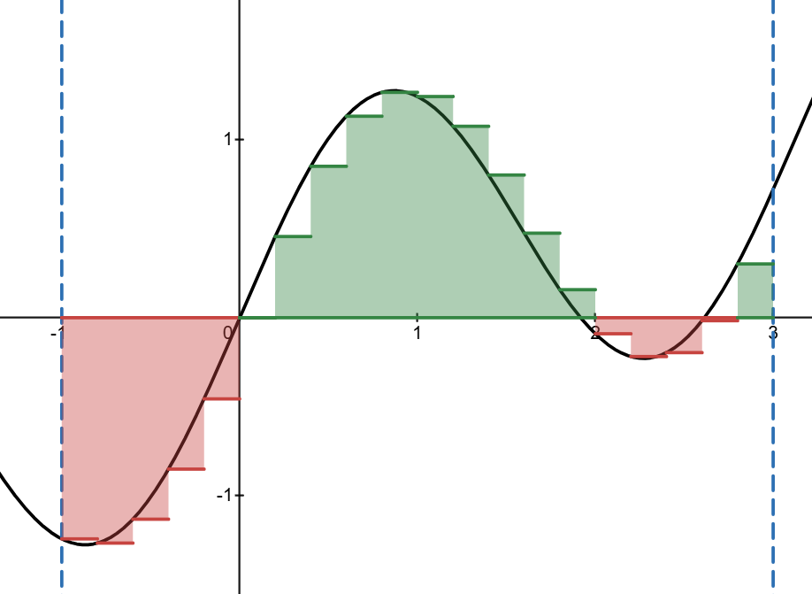
In a Riemann sum, we can have as many or as little rectangles as we want to approximate the function. My question is, is it possible to use rectangles to approximate the graph of the function with basically $100\%$ accuracy?

In the photo above, we have $20$ rectangles approximating the graph. If we increase the number of rectangles to $50$, we can get the following:

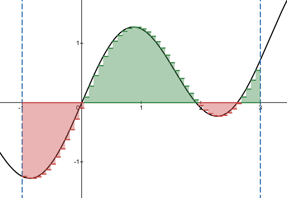
The approximation with the rectangles looks so much better, and there seems to be less gaps.

The general idea is that if we continue to increase the number of rectangles, then we can continue to approximate the graph even more closely until it is perfect.

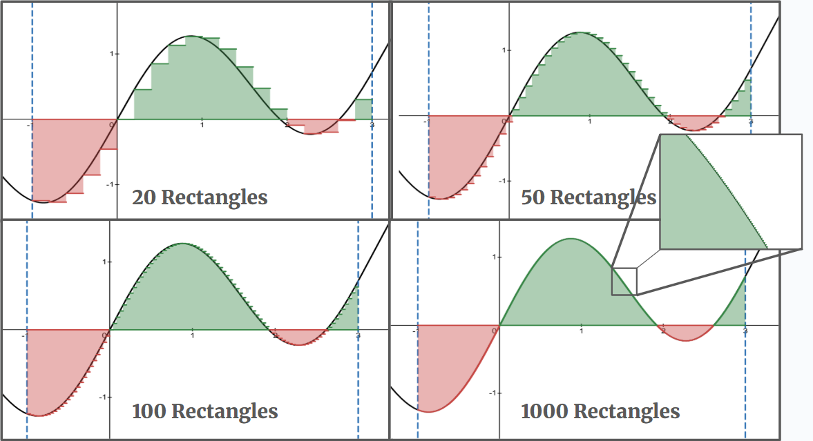
Look at how as we continue to add rectangles, the rectangles get even more accurate until we can’t even see the inaccuracies unless we zoom in! So theoretically, if we had infinite rectangles, we would be able to approximate the area so well that our approximation is the actual area.

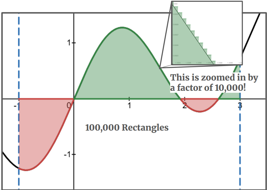
To anyone who is interested, this is what a whopping $100,000$ rectangles looks like. There are basically zero inaccuracies unless you zoom in really far in.

This is all very cool, but how do we actually represent this mathematically? Well, let me introduce you to the summation!

$\sum _{i=1}^{4}i=1+2+3+4$

The general idea of the summation is that you plug in each whole number into the variable. For example, the variable $i$ is the variable you start with. Notice that the bottom number of the summation is $1$ and the top number of the summation is $4$, so we go from $1$ to $4$.

$\sum _{i=1}^4{i}^2+4=((1{)}^2+4)+((2{)}^2+4)+((3{)}^2+4)+((4{)}^2+4)$

$=(1+4)+(4+4)+(9+4)+(16+4)$

$=5+8+13+20=46$

Now let’s take a look at this summation!

$\sum _{i=1}^{n}f(x_i^{\ast })\Delta x_i$

If we were to write it out and expand it, it would look a little something like this:

$f(x_1^{\ast })\Delta x_1+f(x_2^{\ast })\Delta x_2+f(x_3^{\ast })\Delta x_3+...+f(x_n^{\ast })\Delta x_n$

Notice how the whole idea doesn’t change. We started from one, and kept going until $n$. What does this all mean though?

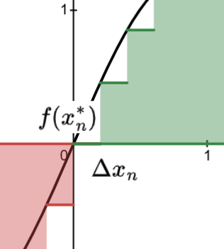
The height of each rectangle can be represented as $f(x_n^{\ast })$, and the width can be represented as $\Delta x_n$. Extend this throughout the entire function, and you will get the result of the summation.

Since we want as many rectangles as possible to make the approximation as close to the actual area, it would make sense for $n$ to be infinity. We cannot actually make $n=\infty$, so we will use a limit instead.

$\underset{n\to \infty }{\lim }\sum _{i=1}^{n}f(x_i^{\ast })\Delta x_i$

This summation would represent the area under the curve perfectly, because we have an infinite amount of rectangles. However, their widths would be nearly zero to make up for that.

Integral Notation

The integral is a mathematical way to represent the area under a curve. For the integral, we have already introduced the notation in Topic 6.1, but let’s go over the notation again.

If we have a function $f(x)$, and we want to find the area under the curve from the interval $[a,b]$, then the integral would look like this:

${\int }_a^{b}f(x)dx$

Notice how the bottom and top of the integral sign represent the interval, and that in front of the integral, we are involving $f(x)$. However, what does $dx$ actually mean? Well, $dx$ is one way to represent an incredibly small value. Let me explain.

Remember the Riemann sums? If we make the rectangles incredibly small, the height will be the function’s value at that point and the width would be incredibly small, making some very thin rectangles. Take this same concept, but make the rectangles infinitely small, the height will be the function’s value but the rectangle’s width will be infinitely small.

If we compare the integral to the summation, notice that $f(x)$ actually represents the height of each rectangle, and $dx$ represents the width of each rectangle.

The Statement

Let’s connect everything together. We have the Riemann sum which represents the approximation of the actual area and the integral which represents the actual area. If we set the Riemann sum to be a perfect approximation, or have an infinite amount of rectangle, we get the following:

$\underset{a}{\overset{b}{\int }}f(x)dx=\underset{n\to \infty }{\lim }\sum _{i=1}^{n}f(x_i^{\ast })\Delta x_i$

We can say that both are equal to each other because they both represent the area under the curve. One of them is a more complicated expression that works, and the other was meant for this situation.

How do we effectively connect the two statements and start plugging in numbers?

Example 1:

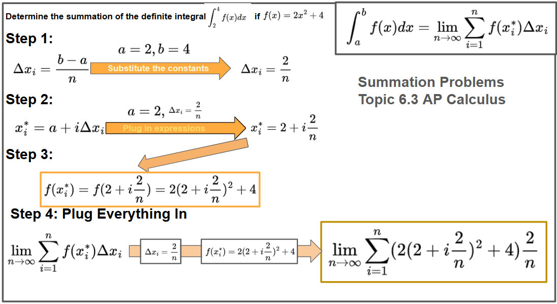
Determine the summation of the definite integral $\underset{2}{\overset{4}{\int }}f(x)dx$ if $f(x)=2x^2+4$.

$\underset{a}{\overset{b}{\int }}f(x)dx=\underset{n\to \infty }{\lim }\sum _{i=1}^{n}f(x_i^{\ast })\Delta x_i$

In this statement, we will have to convert the integral into a summation. We cannot plug in the function directly into the summation because it is in terms of $x$ and won’t do anything useful. Notice that the bottom of the summation has $i=1$, which means that we will have to work with functions that have $i$.

Remember that $\Delta x$ is the width of the function. If we can somehow solve for the width, then we can plug it into the function. If we divide the interval into infinitely many parts, then that would be the width of each rectangle.

We know that $\Delta x_i=\frac{b-a}{n}$. In this case, $b-a$ represents the length of the interval, and $n$ is used because in the summation, $n$ goes to infinity. $n$ also represents the number of rectangles in the approximation, which will go to infinity with the limit in front of the summation. The interval is $[2,4]$ as given by the integral’s bounds, so $4-2=2$. As such, our summation is:

$\underset{n\to \infty }{\lim }\sum _{i=1}^{n}f(x_i^{\ast })\frac{2}{n}$

Now, we will have to define $x_i^{\ast }$. Each input of $x_i^{\ast }$ must represent the height of each rectangle. The first rectangle’s height is at $x=a$ as the first rectangle, and the next one should be $x=a+\Delta x_i$. We add $\Delta x_i$ because that is the width of each rectangle.

The second rectangle will be $x=a+2\Delta x_i$, as we will need to move another $\Delta x_i$ again to determine the height of the next rectangle. If we continue on, we get $x=a+i\Delta x_i$. Remember that the summation is working in terms of $i$, so each rectangle will have a different input that represents each rectangle.

The general formula for the input is $x_i^{\ast }=a+i\Delta x_i$, but remember that $\Delta x_i=\frac{2}{n}$ and $a=2$ from earlier, so our input is actually $x_i^{\ast }=2+i\frac{2}{n}$. We can plug this into the summation.

$\underset{n\to \infty }{\lim }\sum _{i=1}^{n}f\left(2+i\frac{2}{n}\right)\frac{2}{n}$

If we plug in $2+i\frac{2}{n}$ into the original function, we will get $f(x_i^{\ast })=f\left(2+i\frac{2}{n}\right)=2{\left(2+i\frac{2}{n}\right)}^2+4$. Plugging this into our summation gives us the final result:

$\underset{n\to \infty }{\lim }\sum _{i=1}^n\left(2{\left(2+i\frac{2}{n}\right)}^2+4\right)\frac{2}{n}$

That took quite a while, but the general steps of it are to find $\Delta x_i$, find the general formula for $x_i^{\ast }$, plug it into the function, and substitute everything in.

Example 2:

Write the summation for the approximation of the definite integral of ${\int }_2^{7}g(x)dx$ if $g(x)=3-\ln x$ using 10 subdivisions.

We can do the same thing, except that $n=10$. Remember that $n$ represents the number of rectangles, so if $n=10$, it indicates that the approximation will have 10 rectangles or 10 subdivisions.

Remember that $\Delta x_i=\frac{b-a}{n}$, so plugging in $a=2,b=7,n=10$ gives us $\Delta x_i=\frac{7-2}{10}=\frac{5}{10}=\frac{1}{2}$. We can solve for $x_i^{\ast }$ now.

$x_i^{\ast }=a+i\Delta x_i$, and so plugging in $a=2,\Delta x_i=\frac{1}{2}$ gives us $x_i^{\ast }=2+\frac{1}{2}i$.

$g(x)=3-\ln x$, so $g\left(2+\frac{1}{2}i\right)=3\ln \left(2+\frac{1}{2}i\right)$

Plugging this into the summation, we get:

$\sum _{i=1}^{n}g(x_i^{\ast })\Delta x_i$

$\sum _{i=1}^{10}3\left(\ln \left(2+\frac{1}{2}i\right)\right)\frac{1}{2}$

This is the summation that approximates the definite integral of ${\int }_2^{7}g(x)dx$ if $g(x)=3-\ln x$ using 10 subdivisions.

After this topic, we will have finished Riemann sums and will be moving into integrals more. Now that you know all the Riemann sums you need to know, you can play around with this Desmos calculator and find new patterns in Riemann sums! After doing the practice problems, try experimenting with different functions and different numbers of rectangles and see how Riemann sums work right in front of your eyes!

Desmos Calculator: https://www.desmos.com/calculator/tgyr42ezjq