Introduction
Hey there, and welcome to a new article of AP Calculus! Today, we will be going over integrals again and understanding them more!
Approximating Integrals
Last time, we went over what an integral was, which is the area under the curve. Whenever the curve is negative, the area is negative. Whenever the curve is positive, the area is positive. We used geometry and triangles and rectangles to figure out how to approximate a curve and get an actual value or number we can work with. Today, we will be focusing on using geometry to approximate area.
In the previous article, we used triangles and rectangles to approximate the area of this function. While this did work somewhat well, we need a way to approximate a function that isn’t specific to the function itself. A general way to approximate something would be pretty nice. Let me introduce you to Riemann sums.
Riemann Sums
Riemann sums were made by a guy named Bernhard Riemann and it revolutionized Calculus in a way that we will cover in the next article. Anyways, all you need to know for now is that Riemann sums can help approximate the area under the curve through just rectangles. Let’s take a function and I’ll draw the rectangles to help you understand what I mean.

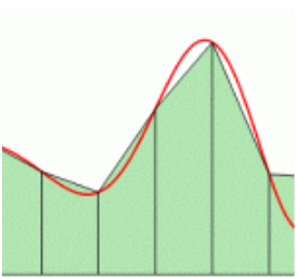
Notice how I use rectangles to sort of trace out the function. Obviously, this approximation doesn’t look very good at all. If I were to increase the number of rectangles I use however, I might get something that looks pretty accurate to the function.
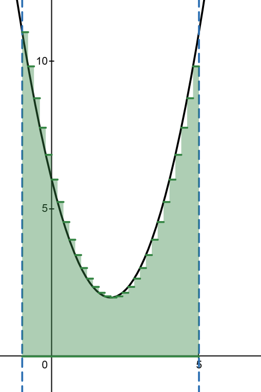
Have a look! I’ve increased the number of rectangles to 30, and the rectangles trace out the function pretty well! Obviously you can see that some rectangles leave some open space while other rectangles stick out, but it doesn’t look half bad!
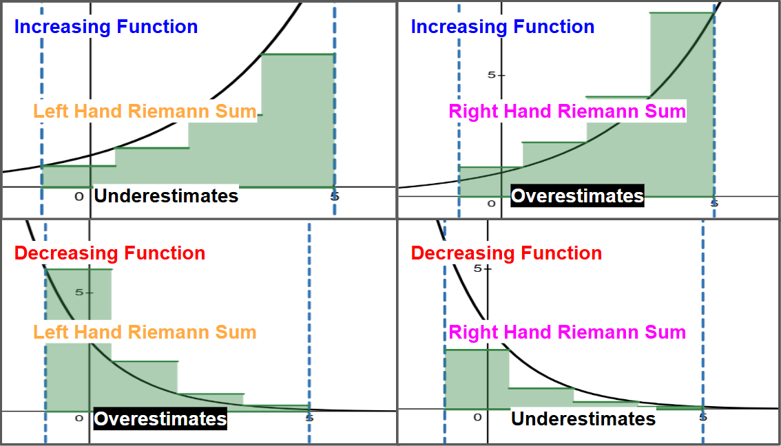
Speaking of sticking out, notice that whenever the function is decreasing, the rectangles always stick out, and whenever the function is increasing, the rectangles always leave some space. Just a little behavior I want you to watch out for!
Types of Riemann Sums
Let’s get into the types of Riemann sums, or ways to approximate a function that the AP Calculus exam needs you to know. Before we begin discussing, I would like to discuss something about the rectangles.
Image 1:
Notice that this is also a valid approximation.
Image 2:
We have two valid approximations of the curve. I’ll admit, not very good ones, but they approximate the curve. Regardless, I think you can spot a very clear difference if you compare the two photos, but what exactly is it? Well, let’s think about a rectangle first.
A rectangle has two sides, a left side and a right side. Notice that for the first image on the top, we used the value on the left side of the rectangle, but the second image used the right side of the rectangle. We have two different Riemann sums, and I think there is a pretty logical name for both of them.
In Image 1, we can call that a left Riemann sum, indicating that it uses the value of the rectangle on its left side. In image 2, we can call that a right Riemann sum, indicating that it uses the value of the rectangle on its right side.
One more thing I would like to note here. Notice that when the function is decreasing, the left Riemann sum rectangles stick out but the right Riemann sum rectangles leave some space. If we then look at when the function is increasing, the left Riemann sum rectangles leave some space but the right Riemann sum rectangles stick out now. Very interesting
Example 1:
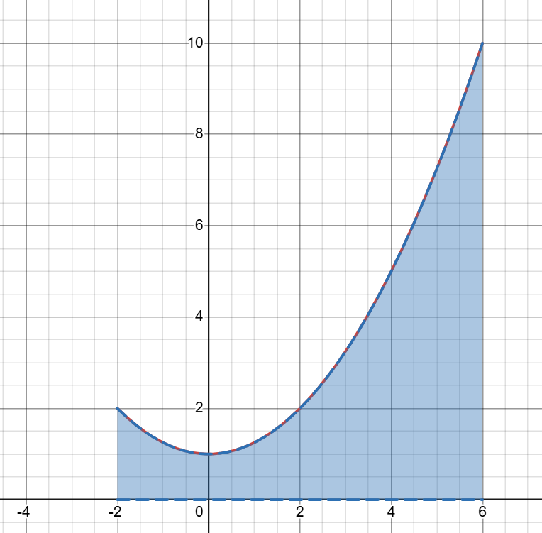
Approximate the area under the curve of the graph shown below in the interval using left and right Riemann sums with 4 equal subdivisions.

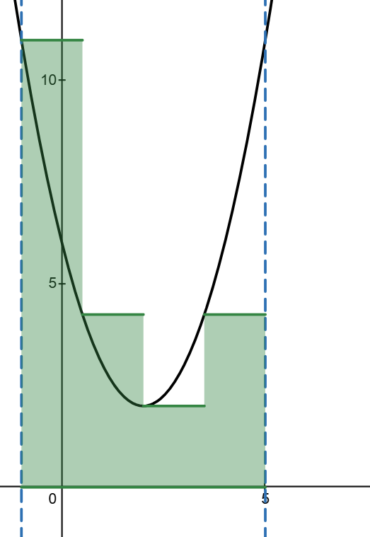
First off, let’s just understand what that last part “with 4 equal subdivisions” means. Whenever it says this, it basically means that you are going to be using four rectangles that are of equal size. Hence, 4 equal subdivisions. Let’s do a left Riemann sum first.
If we were to split the interval into parts, I think it would make sense for each rectangle to have a width of . The distance between and is , so splitting into parts gives us , some simple division here.
Now, there are quite a few ways you can do a left Riemann sum but what I like to do is start from the left most point and go up in increments of the width. Let me demonstrate. First off, the leftmost point is . The -value tells you the height of the rectangle. Since we know that the width is and the height is , that means that the area of the first rectangle is . Let’s move to the next rectangle.
I think it would make sense for the next rectangle’s height to be dependent on the -value at . We just used the -value at for the previous rectangle’s height, so jumping by two (which is also the width of each rectangle), we get that the height of the second rectangle is . Multiply that with the width which is , and you will get that the area of the second rectangle is .
It would take a while to write out the thought process for each rectangle, so I will give you the unsimplified equation for a left Riemann sum. I think you can see a pattern with the function values and the heights of the rectangles.
Each term corresponds to one rectangle in the left Riemann sum.
This is going to be the estimated area under the curve if you used a left Riemann sum. Now, let’s do the right Riemann sum.
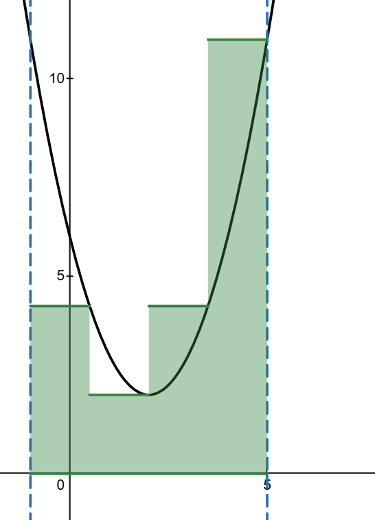
Just like how I start my left Riemann sums on the leftmost point, I start my right Riemann sums on the rightmost point. The right most point is . Take the -value, and that’s the height of the rectangle. The process is basically the same.
Each term corresponds to one rectangle in the right Riemann sum. Take note that the leftmost term in the expression corresponds to the rightmost rectangle in the Riemann sum.
You may spot a lot of patterns with left and right Riemann sums work, but I’ll leave that up to you. Also, just to address the elephant in the room, the left and right Riemann sums are different! Yes the left and right Riemann sums are different and that is going to happen probably every time. Anywhoo, our left Riemann sum is 20 and the right is 36.
Trapezoidal Sum
Let Let’s learn a new one, shall we? Let’s learn about trapezoidal sum. Just from the name, you can suspect it relates with trapezoids, and you would be absolutely correct!
Notice how we simply are using trapezoids to represent the area under the curve, which is a lot better. Also notice that each trapezoid has a very specific shape. The width is, well, the width, but the height on one side depends on that one side and the height on the other side depends on that other side. It would be a waste if I kept on talking, so doing an example problem will help me explain what I mean.
Example 2:
Approximate the area under the curve of the graph shown below in the interval using trapezoidal sum with 4 equal subdivisions.
We have the same graph with the same interval and everything, just that we need to use a different approximation method. With the trapezoidal method, you can imagine it as a mixture between the left and right Riemann sums.
If we draw the trapezoidal sum of the graph, it would look something like this:
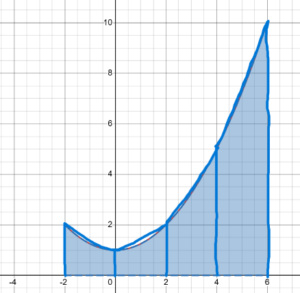
If you remember the formula for the area of trapezoids, it's the height of both ends multiplied by its width divided by 2, or . Let’s look at the first trapezoid. Notice that the height of the trapezoid at both ends is simply the value of the function at and . The width is well, the width, which is . Plugging in our values, we get .
I am not going to go through all the trapezoids, as the way to solve them is essentially the same.
Each term represents one of the trapezoids, and so you can see how each term correlates with what trapezoid in what way.
Here’s just a quick fun fact. Remember the values we got for doing a left and right Riemann sum? The left Riemann sum gave us $20$, and the right Riemann sum gave us . Well… if you add both the left and right Riemann sums and divide them by two, you get the same value as the trapezoidal sum.
Midpoint Sum
Finally, we have reached the last one, and it really isn’t all too different.
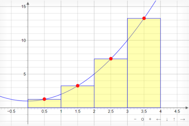
Notice how we still have rectangles and whatnot. Instead of choosing the height of the rectangle to be the left or right, we chose the height of the rectangle in the middle. I think this shouldn’t be very hard to understand, it’s all about the height of the rectangle.
Example 3:
Use left, right, and trapezoidal sums to approximate the area under the curve of the function on the table below in the interval with 4 subdivisions.
Notice how we have everything here except the midpoint sum. Yeah, the midpoint sum only works on functions but not on tables. But anyways, to address the elephant in the room, we have to use a table now to approximate! Don’t worry, it is actually very simple.
There is just one change. Notice that the difference in the -value is changing, hence why the problem doesn’t say “4 EQUAL subdivisions”, just “4 subdivisions” here. Anyways, let’s begin with a left Riemann sum.
For the first rectangle, we can start from the very leftmost point, which is at . The height of the rectangle is the same as the function at , so . If we look at the change in before we get to the next point that we know about, we have a difference of , so it is safe to say that the rectangle is going to have a width of .
Putting together all this information, we have width times height, or . Doing this for all the other rectangles, we get the following:
Each term corresponds to a rectangle. Further simplifying and plugging in numbers gives us:
We can do the same exact thing with the right Riemann sum by starting on the right, which is . Because the next point to the left of us is units away on the -axis, we can safely say that the width of the rectangle is going to be . The height of the rectangle is going to depend on whatever the right side of the rectangle is, so .
Putting everything together, we get the following:
Each term corresponds to a rectangle, where the leftmost term corresponds to the rightmost rectangle. Finishing this off gives us:
We can do the trapezoidal sum now, or… we can do the little trick. Add both the left and right Riemann sums and divide them by two to get .
If you do the trapezoidal sum by yourself, then you will find yourself with the same answer, a little practice for those who want it.
Additional Info
So apparently the AP exam wants you to know that you can solve these using a calculator… great! The AP exam also wants you to know that you can solve these… verbally? Like… using words, man I don’t know. Uhh… well… hmm… oh! The AP exam wants you to know how the approximation relates with the actual value of the function!
I think I should mention again that when you have a left Riemann sum with a decreasing function, you will always overestimate. If you have a left Riemann sum with an increasing function, you will always underestimate. How come? Well, think about it.
In a left Riemann sum with a decreasing function, if the value on the left side is always higher than the right side, the rectangle will be taller than the function itself no matter what. In a left Riemann sum with an increasing function, if the value on the right side is always higher than the left side, the rectangle will be shorter than the function itself no matter what.
Reverse these rules for the right Riemann sum and you got it! Also, there’s no real way to tell if a midpoint sum or a trapezoidal sum overestimates or underestimates unless you compare it with the actual area, or visualize it.