
Introduction
Welcome to AP Precalculus. For many of you, this is your first AP Math class, and I congratulate you for taking this! This is a college-level course that will allow you to skip out of math class when you get to college, and give you an understanding that’ll make you ready for a Calculus course!
Anyways, enough about college credit, let us begin our journey in AP Precalculus by learning about functions!
What is Tandem?
You may wonder, what is “tandem”? It would be quite peculiar for you to learn something that you don’t know the definition of. Tandem can be described as “togetherness”, so the change in tandem would be the “change in togetherness”.
A tandem is also the name of a bicycle that has pedals and seats specifically made for two people to ride on. If you want the bike to move, you would need to move together, and that is the idea of tandem.
Functions
At this moment, you may be asking how the idea of tandem works, so let’s start having correlations.
Think about a function. A function is , and you usually plug things into this function. Whenever you input a number into this function, you receive an output. To put this in a more mathematical way, let’s choose a simple function.
In this function, if you were to input , you would get an output of . If you were to input , you would get an output of , and so on and so on. Notice how when we change the input, the output changes. This is how the tandem, or togetherness works. In this article, you will be learning about all the types of togetherness and change in togetherness.
Graphs
It is also very important that you know what a graph is and know how to read one. A graph has an -axis and -axis which represents the relationship between the independent variable and dependent variable.
Independent variables are your input, and dependent variables are your output. The value of independent variables do not change because of something else in the function, thus the name independent. However, a dependent variable changes because of the independent variable, thus, dependent on something.
Graphs tell you in one picture as to what input gives you what output. For example, take a look at this graph.
I’m sure you’ve looked at a graph before and can tell me what the value of the function is at . The answer is . You should be very familiar with how to read a graph by now.
Interval Notation
To learn domain and range, which is an important topic we will cover soon, we need to know what interval notation is.
, or , or any combination of the parentheses and brackets is an interval. Whenever we use parentheses, we exclude the number from the interval. Whenever we use brackets, we include the number from the interval.
For example, if we were to write , this describes the interval from to . Notice how we do not include the number and instead the “next” number replaces it. This is because of the parentheses symbol next to the . With the , we include it because the bracket is next to the , which means we include the number in the interval.
The is like “and”, so we can sort of “combine” the intervals. The actual name for the symbol is “union”. We will use this symbol soon enough.
Note that in interval notation, whenever we have an infinity, we NEVER use brackets to include it in the interval. There will always be parentheses next to the or because you cannot include , and you cannot include because infinity isn’t a number.
Domain and Range
Oh hey! Would you look at that! We’re at domain and range already, so let us discuss. Before we even start learning about domain and range, I think it would be a good idea to define these terms again from the dictionary.
The domain is defined as an area or territory owned or controlled by a ruler or government. The range is defined as the area of variation between the upper and lower limits on a particular scale.
If we put this into a mathematical context, the domain could be the place the function “controls”, and the range is the highest and lowest -value it reaches. This is very close to what domain and range actually is, and we figured this out with only the English definitions of these words.
Domain describes the values you can input into the function, and range describes the possible values you can get from the function.
Determining Domain and Range
Consider the function . Determine the domain and range of the function.
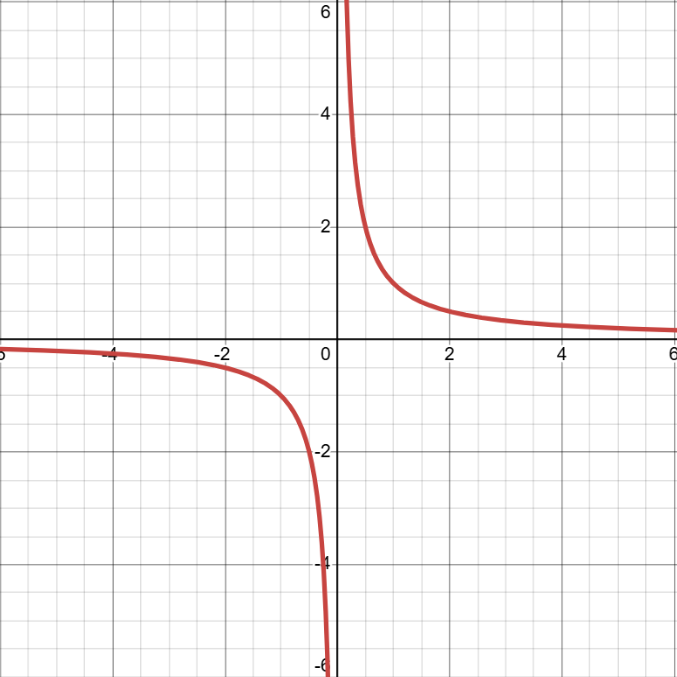
If we were to try to input into , the function would compute , which is undefined. Therefore, is undefined if . At nowhere else is the function undefined, as plugging in any other number will result in a value. This means that the domain of the function is everywhere except at . Also, notice that the function extends both ways all the way to infinity.
The domain of the function can be written as either of the following two.
Domain:
Domain:
To figure out the range, let’s take a look at what output values the function can give. Notice that at , it goes straight down and up both ways. We can reasonably assume that they are going straight down to and . However, if we look both ways left and right, the function seems to be getting closer to . It might reach , but let’s test that theory.If we input into , we get . If we input into , we get . Notice that the function gets smaller and smaller, but it seems to not be exactly zero. Using this information, it is reasonable to think that the range doesn’t include .
Of course, if you have learnt anything about vertical and horizontal asymptotes, this function would be easier to analyze. Regardless, we have figured it out and the range of the function is actually the same as the domain.
Range:
Range:
Remember that you only need to write one of these ranges. Both mean the same thing, just are different ways to write the range.
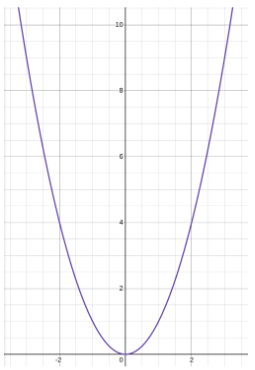
Take note that functions can stay within certain values, for example is shown below.
The function’s range is , as you can input any number into and nothing will go wrong with any of the numbers. The function’s output never exceeds , nor does it go below . The output of can also be any number between, and including, and , therefore its range is .
Increasing vs Decreasing
Consider the two functions below.
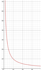
The function is always increasing, as its outputs always increase as the inputs increase. Meanwhile, the function is always decreasing, as its outputs always decrease as the inputs increase. Both functions demonstrate change in tandem, as they change in togetherness, just in different ways. One goes up, and the other goes down.
Formal Definition of Increasing and Decreasing
Although we can simply look at a graph and determine if it is increasing or decreasing very easily, it is also good to get a mathematical sense of what this all means. The definition goes as follows:
Let and be real numbers in the domain of , such that .
A function is increasing if, for all possible values of and , .
A function is decreasing if, for all possible values of and , .
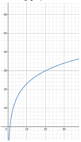
If we have the function @[0, \infty), we can choose numbers of and to prove that this function is either increasing or decreasing. If always, then we can simply plug in these into the function and compare them like this:
,
If is always greater than , then . It makes sense that if you input bigger numbers into the square root function, you will get a bigger output. Thus, the square root function is an increasing function. It should also make sense that this works the other way around, but I won’t go through it.
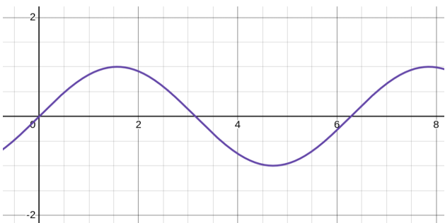
A function can also be increasing or decreasing on an interval. Consider the function .
By just visually looking at the graph, you can see very clearly the intervals at which the function is increasing or decreasing. The function is increasing on the interval , but is decreasing on the interval .
Rate of Change
The rate of change can be thought of as the speed of the function. As the function goes up and down, it will have a steepness. The steeper, the higher the rate of change, and the faster the function goes up and down. This should remind you of slope, which is the rise over run.
Concavity
Concavity is linked with rate of change, and there are two different modes of concavity you can think of. Concave up, and concave down. When a function is concave up, you can think of a cup. The function bends downwards whenever it is concave up. With concave down, you can think of a hill or mountain. The function bends upwards whenever it is concave down.
In a mathematical sense, when a function is concave up, the function’s rate of change is increasing. When a function is concave down, the function’s rate of change is decreasing. It is certainly fascinating that the rate of change… changes!
If you can’t wrap your head around the rate of change changing, let’s look at this with an example. Let’s look at the following table, which represents the miles per hour of a car over a period of 10 seconds.
| Time | Miles per hour |
| 0 seconds | 50 mph |
| 5 seconds | 43 mph |
| 10 seconds | 35 mph |
I would like to point out something very important before we continue. The function that is either concave down or concave up is the TIME vs POSITION graph. In this case, you may notice that this is a TIME vs SPEED graph.
As we can see here, the speed of the car is changing. We can predict if the function is concave up or down just by looking at if the speed is increasing or decreasing. Well, it is certainly decreasing! This means that if we were to graph a time to position graph, we would have a concave down graph.
CollegeBoard expects you to be able to apply this concept to graphs as well. Consider the following graphs.
Concave up is when the rate of change is increasing, and concave down is when the rate of change is decreasing. The idea of rate of change with a graph can be described as the steepness of the graph, so we’re comparing the steepness. If the steepness seems to be getting steeper and steeper, it fits the idea of concave up, and vice versa.
Let’s try this graph now. If we look at the steepness again and compare it from the left to right… Well, let’s see. On the left, the function seems to be pretty steep, but it looks like on the right it slows down and flattens. This matches the description of concave down, so the function is concave down.
Analyzing this function, it’s very steep at the left but it seems to have flattened out. This must mean that the function is concave down. HOWEVER, there is one thing I must say. Notice that the function is going downwards, and this means that the rate of change is negative. Because the function flattens out, the rate of change becomes less negative.
This means that the rate of change went from very negative to less negative, which means that the function is actually CONCAVE UP!
Please do not assume that just because a function gets less steeper, the concavity is down. It is the VALUE of the rate of change that determines concavity.
Similar to what we’ve discussed previously with increasing and decreasing, a function can also be concave up or down on an interval. For example, consider the function .
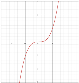
Notice that on the left side of the function, the rate of change seems to be slowing down. This means that it is concave down. The function’s rate of change is positive too, so the rate of change is going from very positive to less positive.
However, on the right side, it seems like the opposite is happening. The rate of change is really slow, but it speeds up and seems to be concave up. The function’s rate of change seems to go from less positive to very positive, so we can confirm that the function is concave up.
Zeros
In our study of tandem and togetherness, you will also have to consider when there is a certain togetherness in the input and output.
A “zero” should be really self-explanatory. A zero occurs when the function or graph hits . In a mathematical sense, the zeros of a function are the input values such that .
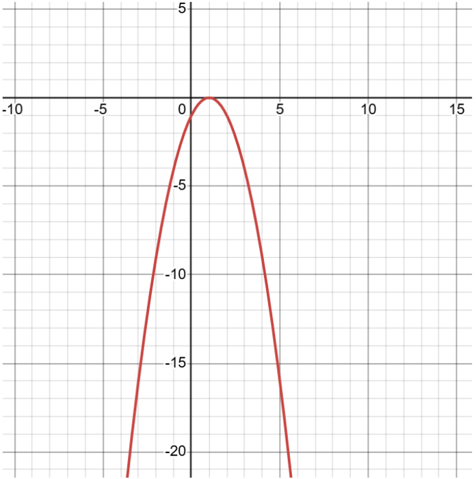
Find the zeros of the function , which is shown in the graph below.
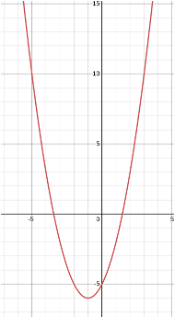
If we simply look at the graph of the function, we can see that the function has zeros at and .
Practice
That is it! There is a lot of content, but this article should give you an understanding of how functions are analyzed through graphs and equations. Now, it is your turn to apply this knowledge!