Introduction

Welcome back to AP Precalculus! Today we’ll be discussing Topic 1.2, which is about the rate of change of a function. While you were likely introduced to this topic in prior math classes, the AP Precalculus curriculum requires that you go more in-depth for this subject! Without further ado, let’s begin!

Review: Rate of Change

In this course, you will be required to know about two different ways to show rate of change, but let’s remind ourselves what a rate of change is. There isn’t a perfect definition for it, but I would say that it describes how much the $y$ value changes in comparison to how much the $x$ value changes.

Imagine that the shape of a graph describes a mountain. If there is a steep part, our left and right movement is relatively low, and we go up very quickly. We can say this is a large rate of change. However, a flatter part means that we go up the mountain more slowly and go left and right faster instead. We can say that this is a small rate of change.

Similarly, imagine this same mountain again. When we are hiking upwards, our rate of change is positive. When we are finished hiking and have to go back down, our rate of change is negative. 

We can apply this same concept to the rate of change. If we have a large change in the $y$-value and small change in the $x$-value, we usually will have a high rate of change. If we have a small change in the $y$-value and a large change in the $x$-value, we usually will have a small rate of change. 

For any other combination (like a large change in $y$-value and a large change in $x$-value), we will have to look at the numbers. Math isn’t an abstract concept, so how do mathematicians define “rate of change?”

Average Rate of Change

You probably learned about the slope of a linear function in your previous math classes. If you remember, slope is defined as the change in $y$ over the change in $x$, or in other words:

$\text{slope}=\frac{\Delta y}{\Delta x}$

If you also remember the slope intercept form, or $y=mx+b$, you may also remember that $m$ was defined as the slope of the function. For example, take a look at the bottom function

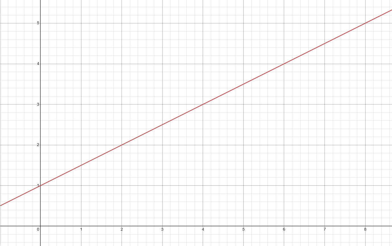
This is a linear function, and the equation of the graph is $y=\frac{1}{2}+1$. How did we even figure this out?

To solve for the slope, we have to consider the change in $y$ and the change in $x$. How do we figure out a change? 

Remember back in 1st or 2nd grade when you did subtraction, and you called it a “difference”. Think about the difference between $5$ and $2$. All you did was do $5-2$ to get $3$. This means that the difference between $5$ and $2$ is $3$. To get a difference, you need to have two different numbers. You can’t be given the number $5$ and be told to find the difference, because there is no difference. Similarly, how would you find the difference between three numbers? 

We can think about difference in the same way here, where difference is the change between values. I would need to change $2$ by $3$ to get $5$, and I would need to change $5$ by $3$ (negatively) to get $2$. In here, we would select two points on the line instead of two individual numbers. You can pick any two distinct points on the line, but we will pick $(2,2)$ and $(6,4)$. 

To find the change in $y$, we simply compare the $y$ values. To solve for the change, we simply subtract the numbers. I think doing $4-2$ is more comfortable than $2-4$, so let’s subtract the second coordinate’s $y$-value by the first. This means that the change in $y$, or $\Delta y$ is 2. 

For the change in $x$, we will do the same thing. Because our change in $y$ is through subtracting the second point’s $y$ value by the first, we will need to solve our change in $x$ by subtracting the second point’s $x$ value by the first. This way, we get the correct answer. $6-2=4$, so the change in $x$, or $\Delta x$ is $4$. 

Going all the way back, our slope is defined as $\frac{\Delta y}{\Delta x}$. We solved for $\Delta y=2$ and $\Delta x=4$, so let’s just plug that in. $\frac{4}{2}=\frac{1}{2}=\text{slope}$. We have finally solved for the slope of the linear line! 

To put this in a more formulaic way. If the change in $y$ is the second coordinate’s $y$ value minus the first coordinate’s $y$ value, then $\Delta y$ = y_2 - y_1$. $y_2$ is just the second (2) coordinate’s $y$ value, and vice versa.

Similarly, if the change in $x$ is the second coordinate’s $x$ value minus the first coordinate’s $x$ value, then $\Delta x$ = x_2 - x_1$. $x_2$ is just the second (2) coordinate’s $x$ value, and vice versa.

This means that $\text{slope}=\frac{\Delta y}{\Delta x}=\frac{y_2-y_1}{x_2-x_1}$. Personally, I trust this second formula more because it literally tells you exactly where to put each number. As long as you know which coordinate is which, it’s as easy as pie.

What about the $+1$? Although it isn't what we need to cover, let’s cover it anyway. This is the $y$-intercept, or the $y$-value where the linear line crosses the $y$-axis. If you look at the graph, you can notice that at $y=1$, the graph crosses the $y$-axis. This means that it intercepts the $y$-axis, or $y$-intercepts at $y=1$. This is why we have a $+1$.

All put together, this gives us the grandiose $y=\frac{1}{2}x+1$

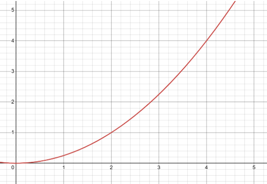
Let’s go back and continue our slope talk. This is indeed one example of rate of change, but this isn’t exactly what we mean by average rate of change. Although it is the average rate of change of the entire function, what about the average rate of change of other functions… say this one:

Well, this isn’t exactly a linear graph. This means that we will be forced to do some average rate of change. If we can’t find an exact change right now, it doesn’t hurt to find an average. 

However, how do we do an average? It’s very weird because if you think about it, the points you choose on this curve matter. It gets steeper and steeper as you go to the right, so how do we know which two points to pick?

Well, typically the question will give you the points to pick, or the interval to solve for the rate of change, so you don’t need to worry about picking, just worry about the solving. Let’s see… how about we solve for the rate of change in the interval $[2,4]$? So from $x=2$ to $x=4$, what is the average rate of change?

Surprise surprise, my fellow mathematicians, we can use the formula we got earlier!  $\text{slope}=\frac{y_2-y_1}{x_2-x_1}$ tells us EXACTLY where to put everything, and so all we need are two coordinates. Another surprise, my fellow mathematicians, we can use the coordinates at $x=2$ and $x=4$! All we have to do right now is simply look at the graph and see.

At $x=2$, the $y$ value is $1$, so our coordinate should be $(2,1)$. At $x=4$, the $y$ value is $4$, so our coordinate should be $(4,4)$. We have our two coordinates! Typically, the rightmost coordinate (the one with a higher $x$ value) is the second coordinate, so let’s just do that. 

First coordinate is $(2,1)$, and second coordinate is $(4,4)$. We can simply follow the formula and get the following:

 $\text{slope}=\frac{y_2-y_1}{x_2-x_1}=\frac{4-1}{4-2}=\frac{3}{2}$

My friends, the average rate of change of this function over the interval $[2,4]$ is $\frac{3}{2}$! Let’s try another one!

If we had no graph, but received the function $f(x)=\frac{3}{x}-1$, what would be the average rate of change over the interval $[1,3]$? Well, we would do the same exact process!

At $x=1$, how do we solve for the $y$ value? Well, we simply just plug $x=1$ into the function, just like we said in Topic 1.1! This means that $f(1)=\frac{3}{1}-1=3-1=2$. This means that the first coordinate is $(1,2)$.

At $x=3$, how do we solve for the $y$ value? Well, same process! Simply plug in $x=3$ into the function to get $f(3)=\frac{3}{3}-1=1-1=0$, so our second coordinate is $(3,0)$.

Combining all our information, we get the following:

 $\text{slope}=\frac{y_2-y_1}{x_2-x_1}=\frac{0-2}{3-1}=\frac{-2}{2}=-1$

This time, the rate of change is negative! How fun!

Instantaneous Rate of Change

Alright, alright. You may or may not remember how I said you couldn’t find the difference between two points, and I’m still correct. This just uses something much more interesting…

Picture this. How do you measure one liter of water? For the cooks and bakers out there, you would probably use those measuring cups. However, does the cup really have one liter of water? I mean, it probably has one liter and three milliliters of water. If you really wanted to follow the recipe exactly, you got to pour out those three milliliters.

After that, you are done, right? Well… nope. You are probably going to spill a little too much and now you’re at $999.53$ milliliters, just under a liter. Remember, the recipe calls for one liter of water. Let’s just… add a little more… and we are still under. Now, we have maybe $999.915$ milliliters… and it’s so close… to one liter…

We can keep repeating this process, but we just can’t detect exactly $1.0000000000000$liters to the utmost maximum precision. At that point, we need to remove or add individual water molecules, and most cooks and bakers don’t have that technology.

Here’s the thing about the instantaneous rate of change. At this moment in time, we don’t have the mathematical tools to actually find an instantaneous rate of change, but we can at least try to get close to it. It’s silly to spill water just because you have $3$ milliliters more water than necessary in a one liter measuring cup, and definitely even crazier to add water when the measuring cup is at $999.53$ milliliters, so let’s just try to approximate an instantaneous rate of change.

Let’s say we have the function $g(x)=\sqrt{(}x)-1$. What is the instantaneous rate of change at $x=4$? Well, we can at least try to choose reasonable values that are somewhat close to it, like $x=1$. We don’t know the exact value of $\sqrt{2}$ or $\sqrt{3}$, and $\sqrt{9}$ is farther away than $\sqrt{1}$. 

Here, we get to choose the points pretty much for ourselves, and so we pick the one at $x=1$ and $x=4$. At $x=1$, the $y$ value can be solved by simply plugging in $x=1$ into the function. $g(1)=\sqrt{1}-1=1-1=0$. The first coordinate is $(1,0)$. 

At $x=4$, the $y$ value is $g(4)=\sqrt{4}-1=2-1=1$. The second coordinate is $(4,1)$. To find the instantaneous rate of change, well… we can’t do that right now. However, our two coordinates here are going to give it their best shot!

Surprisingly, we can still use the slope formula to solve this. Our first coordinate is $(1,0)$, and the second coordinate is $(4,1)$. This means that

$\text{slope}=\frac{y_2-y_1}{x_2-x_1}=\frac{1-0}{4-1}=\frac{1}{3}$

We won’t get into the calculations, but does it make sense that choosing $x=2$ and $x=4$ and finding their coordinates is more accurate? I mean, we are picking points that are closer to $x=4$, and it’s not likely that they stray too far off. If we pick $x=3$ and $x=4$, that approximates the instantaneous slope at $x=4$ even more. Even if we pick $x=3.9$ and $x=4.1$, this is still an insanely good approximation of the instantaneous slope at $x=4$ because of the proximity. 

You don’t need to know how to calculate the instantaneous slope for AP Precalculus, as that is an AP Calculus topic instead (oh how fun!). Rather, first understand that an approximation of the instantaneous slope gets better if we choose points closer to the point of interest. In this case, $x=4.1$ and $x=3.9$ are two very good points to choose because they are near the point of interest, which is $x=4$. 

Eventually, if you have the points close enough, it can give you the instantaneous slope. You can think of these two points being so close to each other that they are essentially the same point. It’s like crushing something so small to the point where it reaches a singularity with basically zero volume. Oh how interesting all this is, but that’s a story for another time.

Wait… why can’t we even solve for instantaneous slopes? Well… here’s the thing. An instantaneous slope is a slope at one point. This means that we would have to find the difference of… one number? And that doesn’t even make sense. You need two distinct numbers to detect a change, but one number? It just doesn’t work out with our current knowledge. 

Oh well. If you’re a junior in AP Precalculus, you will find instantaneous slopes everywhere in AP Calculus. Alright, enough anticipation about the next class you’ll take! I’ll send you off your way and we can have another deep discussion about your high school plans next time! Have a great day, and you should go out to eat some ice cream after doing the practice problems below!

Practice Problems