Introduction

Welcome to the third lesson of AP Precalculus! Today we’ll be discussing topic 1.3, which is about the rates of change in linear and quadratic functions. This topic connects the previous two topics, so you already have some knowledge of what this unit will be about. Here is a quick recap of rates of change…

Recap: Rate of Change

Consider the function $f\left(x\right)=x^2$. If we first consider the two points $(0,0)$ and $(1,1)$, we can see that the AROC is $1$. However, if we consider the points $(1,1)$ and $(2,4)$, we see that the AROC is $3$. The change in AROC between the two different intervals from $[0,1]$ to $[1,2]$ demonstrates how the AROC changes depending on the input variable. This is typical for quadratic functions.

How much is the rate of change changing?

We’ve already covered the rate of change of a linear function versus a non linear function, but we need to discuss how much those rate of changes are changing. While this sounds confusing at first, you’ve probably already learned this, just in a different context. 

Consider a car driving down a road. If it maintains a speed of $20$ mph while it’s driving down the road, then its acceleration is $0$, since its speed is not changing. Meanwhile, if the car speeds up from $20$ mph to $40$ mph, then its acceleration is a positive value, since its speed is increasing. If we were to model the car’s speed as a function, then when we ask how much is the rate of change changing over an interval, we are simply asking for the car’s acceleration over that interval.

Let’s refer back to our previous example of a car going 20 mph down a road. If we were to graph the car’s position, the graph would look something like this.

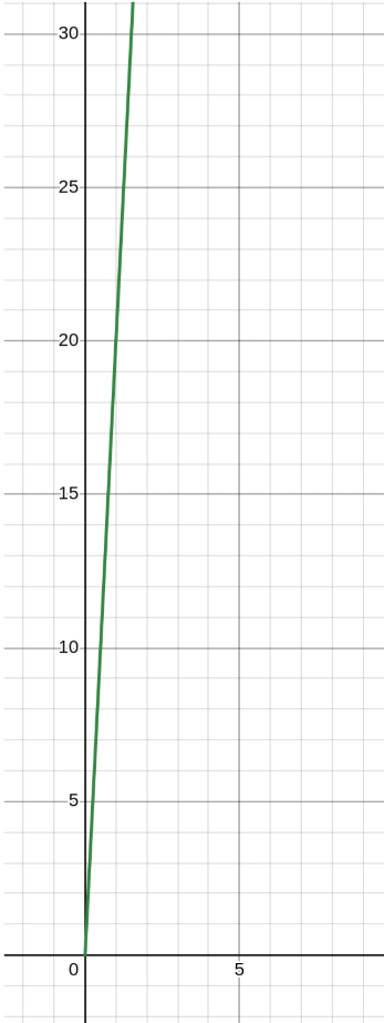
While it certainly is moving at a considerable speed, its speed is always $20$ mph, meaning if we were to graph its speed, it would just be a horizontal line.

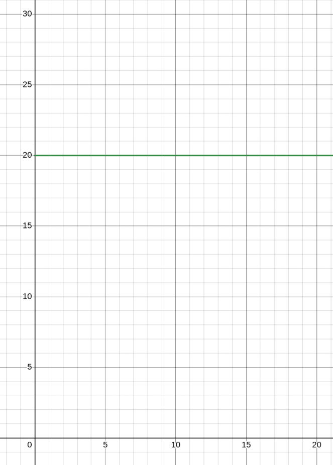
This means that the rate of change is changing at a rate of $0$; it’s not increasing or decreasing.

Compare this to the second example, where the car is speeding up while it’s moving. Since we are only focusing on quadratic functions for this unit, let’s model its position as $y=x^2$ where $x\ge 0$.

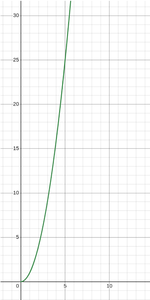
Unlike the previous graph, we can see that our graph’s rate of change is increasing along with $x$. Let’s graph the speed of the car with respect to time and observe the rate of change of this graph.

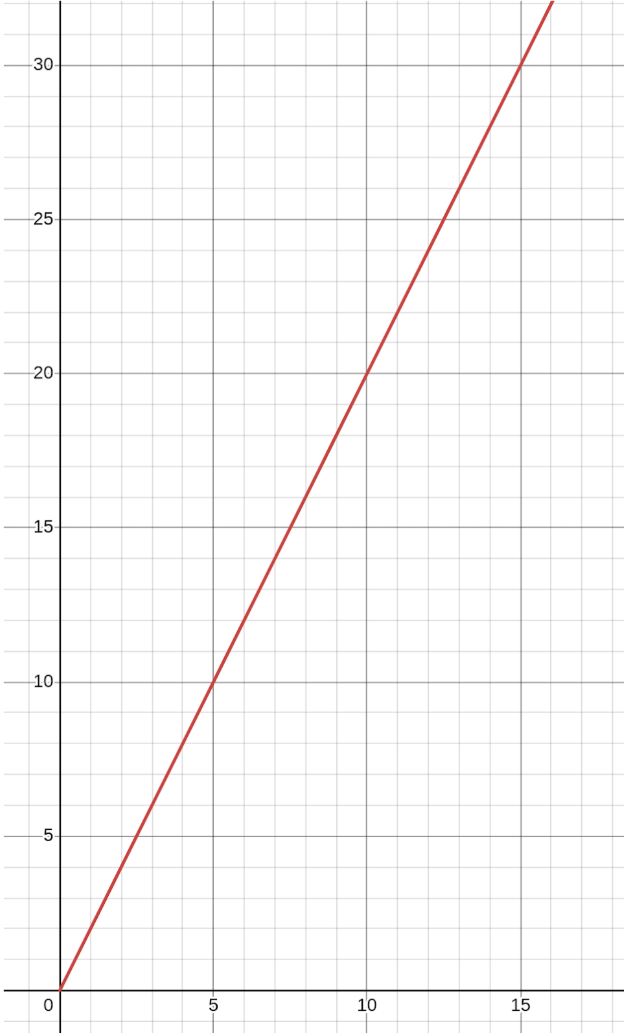
For our function, and also for any quadratic, the rate of change changes at a constant rate.

Concavity

Going back to unit 1.1, the concavity of a function is the direction in which the curve of the function is facing. For example, $x^2$ is concave up, because its curve is facing upwards. The concavity also determines if the rate of change is increasing or decreasing. Since $x^2$ is concave up, as $x$ increases, the rate of change of $x^2$ also increases. This can also be shown in our rate of change graph of $x^2$, where we can see it is increasing at a linear rate.

Now that we’ve discussed the rate of change at a point, we can go more in depth about what it means for the rate of change to be decreasing or increasing. Consider an interval $(a,b)$ and the points inside of it. If the rate of change of each point is increasing as $x$ increases, then the function is concave up and the rate of change is increasing along the interval, and vice versa. Note that I’m not referring to if the rate of change itself is positive or negative since that would correspond with the function’s slope and not the change in the slope.

Practice Problems