Introduction

In this unit, you’ll learn how to decide what kind of function to use to model a given scenario based on data, graphs, or characteristics, and explain the limitations of said choice.

Big Idea

On the AP Exam, you will be given a scenario, a table, or graph, and you must select an appropriate function family (i.e., linear, quadratic, cubic, higher-degree polynomials, or even piecewise functions) and explain why the type of function you chose fits the data. You need to be able to explain what assumptions you make and what implications your choice has on the domain and range.

Data Analysis

Before we begin determining what kind of function best models a scenario, we must understand finite differences–it is a method of detecting the degree of a polynomial function given points from a table, so long as the $x-$values (inputs) are equally spaced.

In the below sections, we will use the following table:

$\begin{array}{ccccccc}x& 3& 6& 9& 12& 15& 18\\ y& y_1& y_2& y_3& y_4& y_5& y_6\end{array}$

First differences

To calculate the first differences, compute $y_2-y_1$, $y_3-y_2$, etc. etc.

If these differences are roughly constant, then the data can be modeled by a linear function, which has a degree of one. 

Note: the suitable error between first differences, which determines whether or not it can be considered roughly constant, will depend on the scale of the numbers.

For example, if you’re measuring distances between planets and you have one million miles compared to one million and five miles (as your first difference), it is roughly constant, since five is negligible compared to one million. However, if you’re measuring the lengths of ants and you have 10mm compared to 15mm, then this cannot be considered constant, as a 5mm difference is huge (50%) compared to the scale.

A general rule is that if the numbers are within about 10% of each other, they can be considered to be roughly constant; you should always trust your gut, though. On the AP exam, it will be clear whether an error is acceptable, you will never need to guess.

Second differences

The process is similar for second differences. The only difference this time is that you subtract the first first difference from the second first difference. For example, the first term in a second difference would be $\left(y_3-y_2\right)-\left(y_2-y_1\right)$. And, if these differences are roughly constant, then it can be modeled by a quadratic model.

This pattern continues on, we can take successive second differences to find the third differences, and so on.

Function Families

Linear Function

The general form of a linear function is $f\left(x\right)=mx+b$

Linear functions are great at modeling situations in which values change at a constant rate. Common words that describe this are “per”,  “for every,” or anything that implies a constant rate of change.

When looking at a table of values, it implies that while the $x-$values are evenly spaced, the first differences (the difference between consecutive outputs/$y$-values) are roughly constant. Preferably (and usually), they will be exactly constant; however, especially when modeling real life data, having a small bit of error is fine. 

When plotting the points on a graph, you should be able to draw a straight line that is close / passes through each of the points.

Quadratic Functions

There are two general forms of quadratic functions that you will need to know.

The first is standard form: $f\left(x\right)=a{x}^2+bx+c$

The second is vertex form: $f\left(x\right)=a{\left(x-h\right)}^2+k$

Quadratic models are very good at modeling a data set when the rate of change of the dataset itself is changing at a constant rate. The data typically approaches a minimum or maximum, and the rest of the data is symmetrical around that extreme.

In contrast to linear functions, when values of a quadratic function are evenly spaced, their first difference (the difference between output values) is not constant. Instead, their second differences are (roughly) constant.

Alternatively, you could also graph the data, and, if it is best modeled by a quadratic, it will resemble a parabola with exactly one vertex (one single peak or valley).

Cubic Functions

Cubic functions take on the general form $f\left(x\right)=a{x}^3+b{x}^2+cx+d$

Typically, the only applied scenario (anything other than raw data points) you’d best use a cubic function to model is in the context of a volume problem or scaling in three-dimensions.

The best way to be sure is to just look at the values in a table. For cubic functions, when the inputs, $x$, are equally spaced, neither the first nor second differences are constant. Rather, the third differences should be roughly constant.

Things become much more ambiguous when looking at it graphically, so it’s not recommended. However, one possible indicator that a dataset is best modelled by a cubic function is if it changes from increasing to decreasing or decreasing to increasing two times. Another indicator, though not perfect (as any function with an odd degree will also exhibit this behavior), is the end behavior of the function: $\underset{x\to \infty }{\lim }f(x)\ne \underset{x\to -\infty }{\lim }f(x)$ if the $f(x)$ is cubic.

Higher-Degree Polynomial Functions

From 1.4, you know that a polynomial function will take on the general form 

$f\left(x\right)=a{x}^n+b{x}^{n-1}+...+c{x}^2+dx+e$

Usually, at most, you will be tested on Quartic or Quintic functions (fourth and fifth degree).

The easiest way to tell if data is best modeled by a polynomial is just by looking at the graph. If the graph has multiple real zeros, or if there are several local maxima/minima (more than a quadratic or cubic would produce), or any other traits unique to a high-degree polynomial (which are explored in greater detail in article 1.4 on FiveHive), the data is likely best modeled by a polynomial function with a higher degree.

When looking at a table of values, it becomes slightly more complicated. When inputs are equally spaced, the n-th differences should be roughly constant (and nonzero), if a polynomial of n-th degree best models the data.

The main takeaway, though, is that polynomial functions best model data when there are multiple local max/mins, multiple zeros, or when the n-th differences point to a degree higher than $3$.

Piecewise Functions

A piecewise function uses different formulas on different (nonoverlapping) intervals of the domain. There is not exactly a general form, but an example could be:

$f(x)=\{\begin{array}{ll}g(x),& x<a\\ h(x),& x\ge a\end{array}$

It is difficult to make a general rule for piecewise models. Often, the best way to figure out the behavior of a piecewise function is to find a point where the behavior of the graph changes.

More informally, if the graph looks “broken,” then it’s most likely a piecewise function. Some clear signs of this is if there is a point at which the function is not continuous or if there’s a sharp corner at a specific point.

From there, you can separate the graph into multiple sections, where each section represents an individual case of the piecewise function.

You can use piecewise functions to model a scenario when one function is not enough to describe the entire dataset.

For example, a piecewise function may be used when modeling parking rates, calculating shipping/payment costs, or calculating how much taxes someone owes.

Geometric clues

Many geometric models can be guessed simply from the dimension. 

For example, in two-dimensional (area) contexts, the best way to model an area is usually a quadratic, and for three-dimensional (volume) contexts, the best way to model volume is usually a cubic (which will be expanded on in the next section). This is because, often, the area of a 2D shape is proportional to a quadratic, and the same applies to 3D objects and cubics. However, especially for irregular shapes, this isn’t always the case.

Regressions

If you want a full Desmos guide from FiveHive, check out the AP Precalculus Desmos Guide

Once you’ve decided on a type of model (linear, quadratic, cubic, etc.), Desmos (which will be provided to you on the exam), or your graphing calculator (if it has a regression option) can help you find the exact best–fit equation for your data through a process called regression.

Typically, regression will exclusively be used for when you are given data points

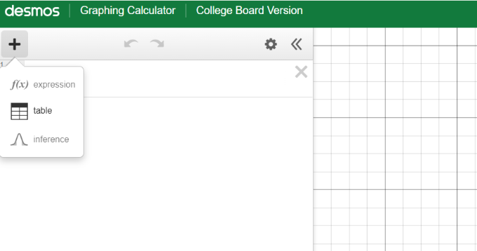
First, open up the Desmos Graphing Calculator. The version that is on desmos.com is slightly different than the one in BlueBook, but any changes present are minor.

Click the “+” → Table to create a data table

Then, enter your inputs in the first column (Desmos labels it $x_1$) and outputs in the second column $y_1$

Then, we can input the regression.

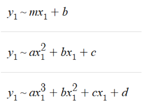
In Desmos, regressions use the tilde symbol (~). It should be found above your tab key (press shift + `). Using the general forms that we listed above (other than for piecewise functions, in which you must separate the graph into their own unique behaviors), we can create a regression. 

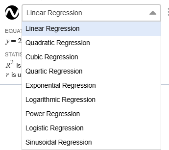
Alternatively, you can click the regression button:

From here, choose the best regression using the dropdown menu

For each regression, you will receive some data

For this unit, all we care about is $R^2$. 

To understand what its significance is, let’s interpret the regression. The equation Desmos is giving you is the “best fit” within the model you chose (linear, quadratic, etc.). A higher $R^2$ means that the function fits the data better (with a max $R^2$ of 1). If I had used a quadratic function to model my data instead, my $R^2$ would be significantly lower and thus imply that the quadratic model does not fit my data well.

Additionally, the function that Desmos provides you can be used to estimate data at points between the data given.

You will learn later, though, that a high $R^2$ may not always mean a great fit, and instead, you will learn how to use residuals to determine how well a function fits.

Assumptions and Restrictions in Modeling

When we model data, it is almost never a perfect prediction. Rather, it is a simplified version that emphasizes an overall trend with the data.

Articulating Assumptions

Consistency Assumptions

These are assumptions about what is considered constant when we use a model. It’s essentially what we consider doesn’t change.

For example:

While these often aren’t constant in real life, we model them as constant in order to reflect general trends in the data.

Covariation Assumptions

Covariation assumptions describe how quantities change together. It explains how if one variable changes, how the other responds.

For example:

Covariation assumptions are important because you are justifying why you chose a specific model for your data.

Domain Restrictions

Speaking from a purely mathematical perspective, a polynomial is defined for all real numbers.

However, in the real world, the dataset that a function models is not defined for all real numbers. You will almost always restrict the domain based on multiple factors, including:

Context clues/implications:

Take time, for example. You cannot have a negative time, for that wouldn’t exactly make sense. The point in which you start something is considered time equals zero. As a corollary, time is considered to be greater than or equal to zero $t\ge 0$.

The same restriction applies to physical quantities such as length, area, volume, mass, # of things (people, animals, etc.), etc. They must all be nonnegative.

Validity Range / Extreme Values

Sometimes, a model only makes sense within the data range used to build it.

In fact, FRQ 2 on the AP exam for AP Precalculus almost always tests this; it specifically asks if a model can be accurate at a time outside of the given data. They will give you a scenario in which the real life data does not match the model, and you must explain why the error is increasing. 

Predicting beyond the data (extrapolation) can give unreasonable results, so you must restrict the domain to the observed interval.

A common type of problem involving this is with a box from a sheet of cardboard:

Let $V\left(x\right)$ be the volume of an open-top box formed by cutting squares of side x from the corners of a rectangular sheet.

There are two implications we must consider. 

If a sheet as a width $w$, a reasonable domain would be: $0<x<\frac{w}{2}$ (in reality, $x$ may have an ever smaller upper bound based on the length)

Discrete vs Continuous

Discrete means that a function has values that exclusively occur at distinct, countable points. (think the number of students in a class; you can’t have 2.5 students. Rather, you have 20, 21, or 22 students)

Continuous means that a variable can take on any value within an interval (the height of a student could be 5.6ft tall, 5.7 ft tall, etc.)

If the dataset contains discrete values, you’ll often round your model to an integer. For example, if you have a question asking you how many years it takes for a sample of radium-226 to decay to one half its original amount (where you for some reason need to give your answer as a whole number), and you calculate it to be $1599.1$, you would round it to $1600$ years. If you were to round it to $1599$ years, then it would not have reached half of its mass yet. Only after $1600$ years has it actually reached half of its mass.

However, for a problem like counting bacteria that have been cultured, if you obtain a number like $54.7$, then you’d round it to $54$ since you haven’t yet formed the 55th bacterium. 

How to approach Modeling Questions

First, read the above in order to find a function type that makes sense for your data. Then, check if your function makes sense in the context of the problem: for example, if you’re modeling the height of a water droplet shot out of a water gun, does your function first increase then decrease? You should also make sure that your model isn’t overcomplicated: a quintic function is likely not necessary for simple data.

Some additional things you can do are 

Practice Problems

1) An AP Physics C student measures the distance of a moving object at various time intervals. The data is shown in the table below.
$\begin{array}{ccccc}t(\text{seconds})& 1& 2& 3& 4\\ d(\text{meters})& 10.2& 20.1& 30.5& 39.8\end{array}$
If the student were to graph distance vs time on an $xy$-plane, what type of model would be most appropriate for this data? Explain why.

2) A student wants to model the mass of a solid, uniform (meaning, density is a constant $\frac{\text{mass}}{\text{volume}}$), steel sphere as the radius of the sphere increases. The student has data comparing various radii with their corresponding mass of the sphere. The volume of a sphere is $\frac{4}{3}\pi r^3$. Without performing calculations, what function would be most appropriate to model this scenario? Explain briefly.

3) A tutor charges a flat $$50$ fee to tutor for one hour, and then charges an additional $$30$ for every hour they continue to tutor. Create a function that would best model this situation.

4) You are modeling the volume $V$ (in $m^3$ aka meters cubed) in a tank as it drains over time $t$ (in minutes). The scenario is depicted in the picture below (NOT DRAWN TO SCALE). Each side of the rectangular tank is $2m$ long. Water drains from the tank through a nozzle located on the side of the tank.

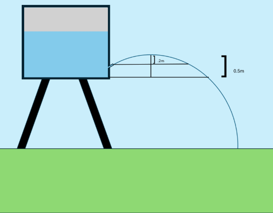
A set of data comparing time $t$ to volume $V$ is collected while the tank is draining.

$\begin{array}{cc}\text{Time }t(\text{minutes})& \text{Volume }V(\text{meters cubed})\\ 0& 14.4\\ 2& 10.0\\ 4& 6.4\\ 6& 3.6\\ 8& 1.6\end{array}$

What function family best models the relationship between time and volume? Justify your answer.

Write out the appropriate regression model to create a function $V\left(t\right)$ that models the volume of the water remaining in the tank.

What is the volume of the water at $t=9$?

Answers

1)  An AP Physics C student measures the distance of a moving object at various time intervals. The data is shown in the table below.$\begin{array}{ccccc}t(\text{seconds})& 1& 2& 3& 4\\ d(\text{meters})& 10.2& 20.1& 30.5& 39.8\end{array}$
If the student were to graph distance vs time on an $xy$-plane, what type of model would be most appropriate for this data? Explain why.

Answer:

A linear model. Because we are given tabular data, we first check if values of time are equally spaced; they are (increasing by $1$). This allows us to use Finite differences.

First, calculate the First Differences by subtracting consecutive outputs $y_2-y_1$.

$20.1-10.2=9.9$

$30.5-20.1=10.4$

$39.8-30.5=9.3$

These can be considered roughly constant (even the variance of $9.3$ from $10.4$ still falls around the 10% rule)

Because the first differences are roughly constant, a linear model is appropriate.

2) A student wants to model the mass of a solid, uniform (meaning, density is a constant $\frac{\text{mass}}{\text{volume}}$), steel sphere as the radius of the sphere increases. The student has data comparing various radii with their corresponding mass of the sphere. The volume of a sphere is $\frac{4}{3}\pi r^3$. Without performing calculations, what function would be most appropriate to model this scenario? Explain briefly.

Answer:

A Cubic Function

First, let us identify the context. The problem relates the mass of a solid sphere to the radius.

We can refer to the geometry to decide our function. From the problem, we know that $\text{Density}=\frac{\text{Mass}}{\text{Volume}}$. Rearranging, $\text{Density}\cdot \text{Volume}=\text{Mass}$. Thus, Mass is directly proportional to Volume.

And, for any three-dimensional (volume) contexts, the best model to model volume is usually a cubic, when we’re relating volume to a variable cubed. Substituting volume in, we get that $\text{Density}\cdot \frac{4}{3}\pi r^3=\text{Mass}$, implying that Mass is directly proportional to radius cubed. Thus, the relationship between Mass and Radius for this scenario is Cubic.

3) A tutor charges a flat $$50$ fee to tutor for one hour, and then charges an additional $$30$ for every hour they continue to tutor. Create a function that would best model this situation.

Answer:

$f\left(t\right)=30t+20$ where $t\ge 1$, or $f\left(t\right)=50+30\left(t-1\right)$.

Both of which, only work when t is a whole number

First, let’s analyze some context clues/words: “additional $$30$ for every hour” implies the rate of change. Just by looking at the phrase “every hour” we can assume it’s a linear function, where the slope is $30$.

The problem states that it costs “$$50$ fee to tutor for one hour.” So, we obtain the point $\left(1,50\right)$. 

Now, we have two points and can simply create our linear function, which comes out to be $f\left(t\right)=50+30\left(t-1\right)$ in its raw form.

It is good practice to check our answer; when we plug in one, we should get $$50$, which we do.

When we plug in two, we should get $$80$ ($50$ for flat fee and a $30$ additional), which we do.

4) You are modeling the volume $V$ (in $m^3$ aka meters cubed) in a tank as it drains over time $t$ (in minutes). The scenario is depicted in the picture below (NOT DRAWN TO SCALE). Each side of the rectangular tank is $2m$ long. Water drains from the tank through a nozzle located on the side of the tank.

A set of data comparing time $t$ to volume $V$ is collected while the tank is draining.

$\begin{array}{cc}\text{Time }t(\text{minutes})& \text{Volume }V(\text{meters cubed})\\ 0& 14.4\\ 2& 10.0\\ 4& 6.4\\ 6& 3.6\\ 8& 1.6\end{array}$

What function family best models the relationship between time and volume? Justify your answer.

Write out the appropriate regression model to create a function $V\left(t\right)$ that models the volume of the water remaining in the tank.

What is the volume of the water at $t=9$?

Answer:

Part A: Quadratic Function

Once again, we have Tabular data. So, let’s first check if the inputs are equally spaced: they are (by $2$). We can use Finite Differences because of this.

Calculating the first differences,

$10.0-14.4=-4.4$

$6.4-10.0=-3.6$

$3.6-6.4=-2.8$

$1.6-3.6=-2.0$

The first difference is not constant. Thus, we move onto the Second Difference.

$-3.6-(-4.4)=0.8$

$-2.8-(-3.6)=0.8$

$-2.0-(-2.8)=0.8$

The Second differences are exactly constant, so a quadratic function is the best fit.

Note, if you said cubic because you saw volume, remember, that is only true when we compare something like side length or radius to volume. Here, we are comparing time, which does not have a cubic relationship to Volume (explained in the notes; also the reason why “usually” is stated).

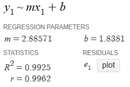
Part B:

$V\left(t\right)=0.1t^2-2.4t+14.4$

Here, we simply used the regression available on Desmos (Desmos SAT Graphing Calculator) by plugging in our data points and using a Quadratic Regression.

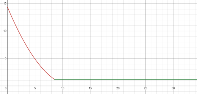
Part C: $1.2m^3$

First, we must consider the range of our function. Our max volume is at $t=0$, since that is when we begin measuring. However, notice that the nozzle of the water tank is not located at the bottom of the tank. In fact, it is located $0.5-0.2=0.3$ meters above the tank. From here, we can calculate the amount of water that will stay in the tank (the minimum amount of water in the tank). Since we know that each side of the tank is $2$ meters, the volume of the bottom portion of the tank (below the nozzle) is $0.3\cdot 2\cdot 2=1.2$. Thus, our minimum volume of water is $1.2m^3$. If we had immediately plugged in $t=9$, we would have gotten the answer $0.9m^3$, which is not physically possible. Rather, past $t=8.54$, the function flatlines, as shown below: