Introduction

Welcome! In this lesson, we’ll focus on logarithmic functions in context and how they are used for data modeling. Building on your understanding of exponential functions, you’ll see how logarithmic functions act as their inverses and help describe situations involving proportional growth or repeated multiplication. You’ll learn how to construct logarithmic models using proportions, input-output pairs, transformations, and technology-based regressions. By interpreting numerical results in real-world contexts, you’ll use these models to analyze data and make predictions about dependent variables.

Essential Knowledge from the CED

According to the AP Precalculus Course and Exam Description (CED), these are the key ideas you’ll be expected to understand about exponential functions for the exam:

Logarithmic Functions as Inverses of Exponential Functions

Logarithmic functions are the inverses of exponential functions, which means they reverse exponential growth. Exponential functions show how a quantity grows by being multiplied by the same factor over and over, while logarithmic functions tell us how many times that multiplication happens. Because of this, logarithmic functions are useful for modeling proportional growth instead of constant change.

In logarithmic models, equal increases in the output match proportional changes in the input. This means the input does not increase by the same amount each time, but by the same factor. When the output of a logarithmic function is a whole number, it shows how many times the original value was multiplied by a constant factor. This helps explain real-world situations where growth is fast at first and then slows down.

Let’s look at an example!

$\begin{array}{cccccc}x-\text{values}& 1& 3& 9& 27& 81\\ y-\text{values}& 0& 1& 2& 3& 4\end{array}$

As you can see here, the x-values are increasing by a factor of $3$ each time, not by adding the same number. Each time the $x-$value is multiplied by $3$, the $y-$value increases by $1$. This shows a logarithmic relationship modeled by $y={\log }_3(x)$. The $y-$value tells us how many times $1$ must be multiplied by $3$ to reach the given $x-$value. 

Constructing a Logarithmic Model from Given Information

A logarithmic function model can be created when key information about a situation is known. One way is by using a known proportion and a real zero. For example, suppose a bacteria culture starts with $1\mathrm{bacterium}$ and triples every hour. We can track the growth in a table:

$\begin{array}{cccccc}\text{Bacteria }(x)& 1& 3& 9& 27& 81\\ \text{Hours }(y)& 0& 1& 2& 3& 4\end{array}$

From this table, we can see that each time the bacteria count triples, the number of hours increases by $1$. This situation can be modeled by the logarithmic function: $y={\log }_3(x)$

Another method is using two input-output pairs. For example, consider sound intensity:

$\begin{array}{ccc}\text{Sound }(x)& 10& 100\\ \text{Intensity }(y)& 1& 2\end{array}$

From this table, we can see that increasing the sound by a factor of $10$ increases the intensity by $1$. This pattern can be modeled by the logarithmic function: $y={\log }_{10}(x)$

Building Logarithmic Models Using Transformations

We can create logarithmic models by starting with the parent function: $f(x)=a{\log }_b(x)$

Transformations let us adjust this basic function to match real-world data. The main types are:

Example:

Suppose we are modeling how long it takes a car to slow down depending on the braking force applied. Assume that the time it takes to stop can be modeled as $f(x)=a{\log }_{10}x+b$. From the data, we notice:

We can write the transformed model as:

$f(x)=2{\log }_{10}(x)+2$

$\begin{array}{cccc}\text{Braking force }(x)& 1& 10& 100\\ \text{Time to stop }(y)& 2& 4& 6\end{array}$

As you can see in the table, multiplying by $2$ makes the time increase faster as braking force increases, and adding $2$ accounts for the minimum $2\mathrm{second}$ delay. This shows how transformations adjust the parent logarithmic function to match real-world data.

Using Technology and the Natural Logarithm to Model Data

The natural logarithm function, $\ln x$, is often especially useful for modeling real-world phenomena. It is helpful for situations involving continuous growth or decay, like populations, chemical reactions, or other processes that change proportionally over time. Logarithmic models can then be used to predict values of the dependent variable.

A useful calculator that can be used and which you have access to on the AP exam is Desmos. This allows you to enter data and perform logarithmic regression, which finds the logarithmic function that best fits a set of data points.

Let’s look at an example:

Suppose a scientist is tracking the concentration of a medicine in the bloodstream over the first few hours after it is administered. The data collected is:

$\begin{array}{ccccc}\text{Time (hours) }(x)& 2& 4& 8& 16\\ \text{Concentration (mg/L) }(y)& 20& 48& 65& 85\end{array}$

First, we have to find the regression of this model using technology. This will give the logarithmic function that best fits the data and can later be used to predict the concentration at times not recorded in the table.

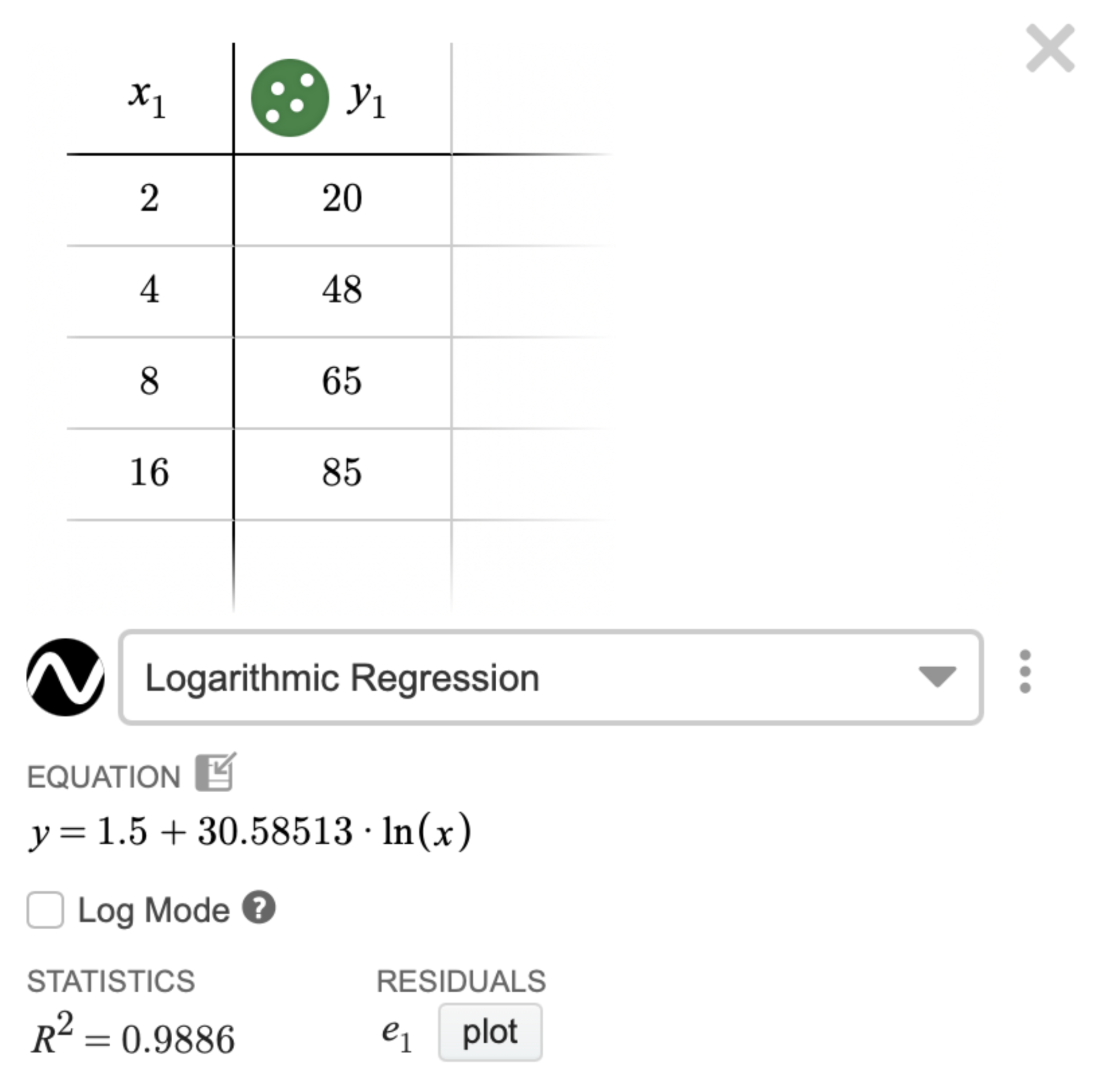
Let’s say we want to figure out what the concentration of the medicine would be after $10\mathrm{hours}$. Once we have the logarithmic regression function, we can simply plug in $x=10$ to estimate the concentration at that time. This shows how logarithmic models allow us to make predictions based on the pattern of the data.

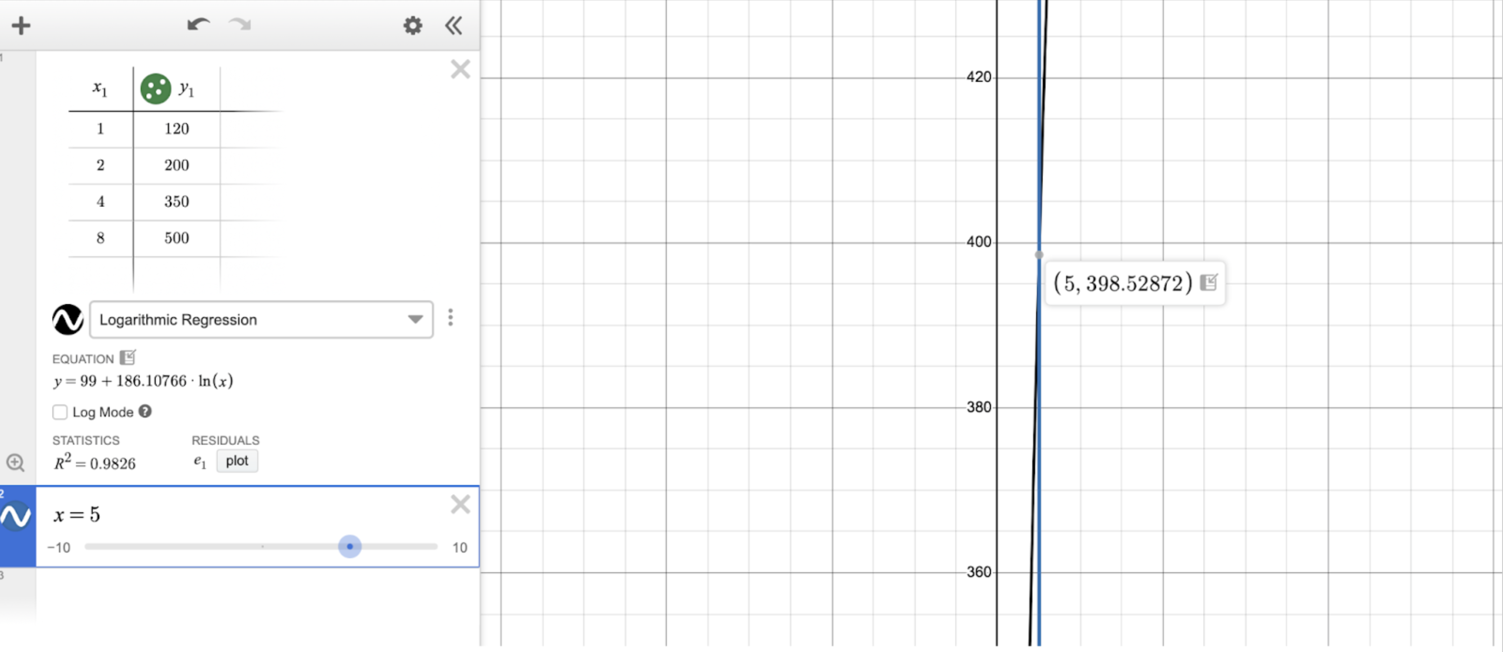
We can type $x=10$ into Desmos and then, by looking at the vertical line at $x=10$, see where it intersects the graph. That intersection point will give us the estimated concentration at $10\mathrm{hours}$.

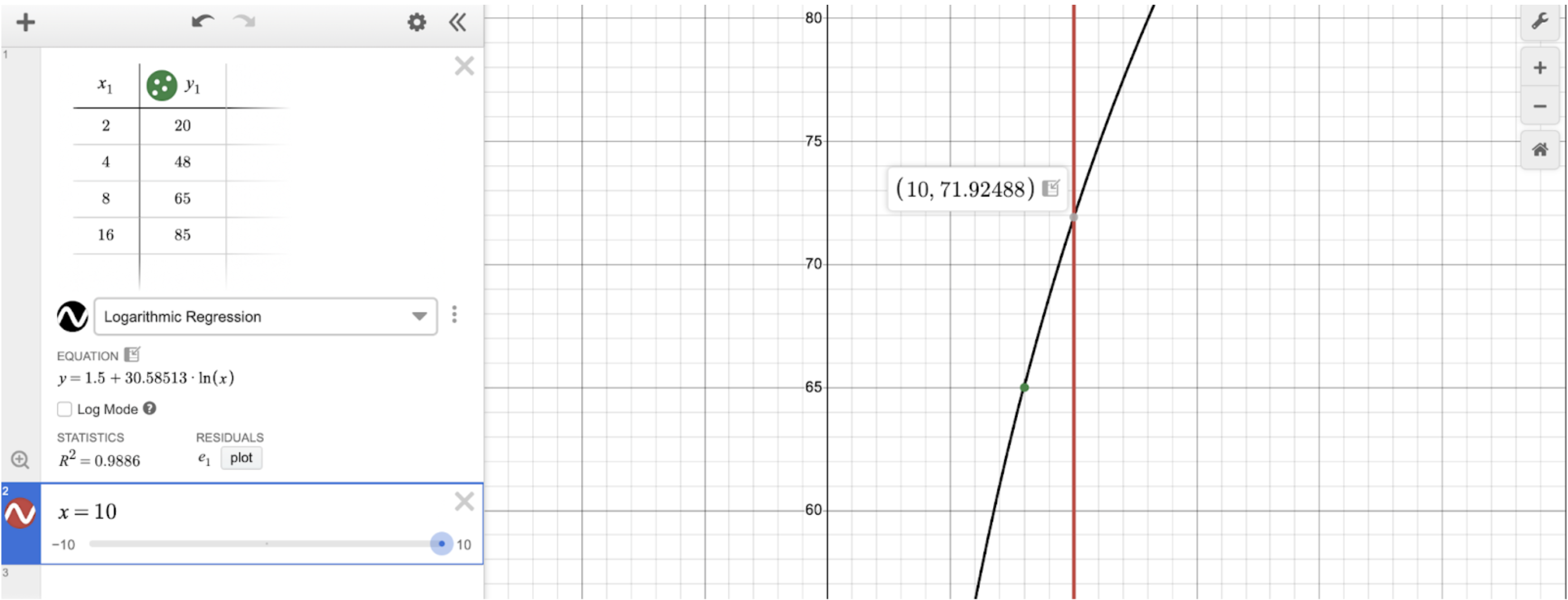
The line $x=10$ intersects the graph at the $y=71.92488$. For the AP exam, rounding to three decimal places, the concentration of the medicine at $10\mathrm{hours}$ is approximately $71.925mg/L$.

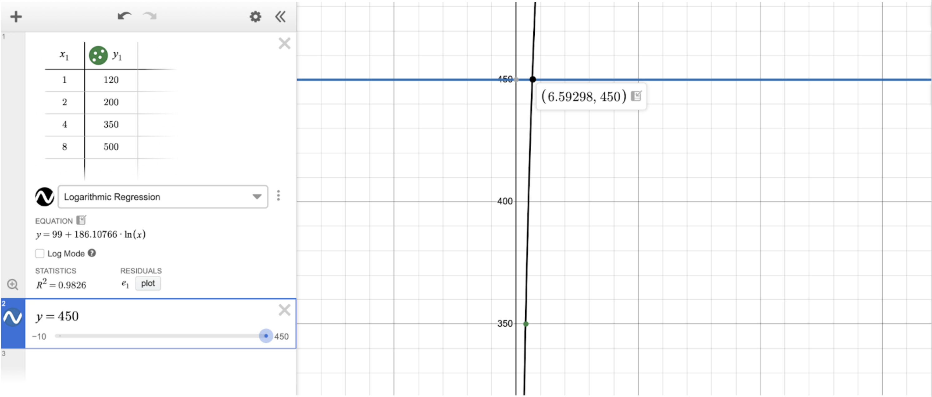
Let’s say we wanted to figure out when the concentration reaches a specific value, like $50mg/L$. Using the regression graph in Desmos, we can draw a horizontal line at $y=50$ and see where it intersects the curve. The $x$-value of that intersection will give us the approximate time when the concentration reaches $50mg/L$.

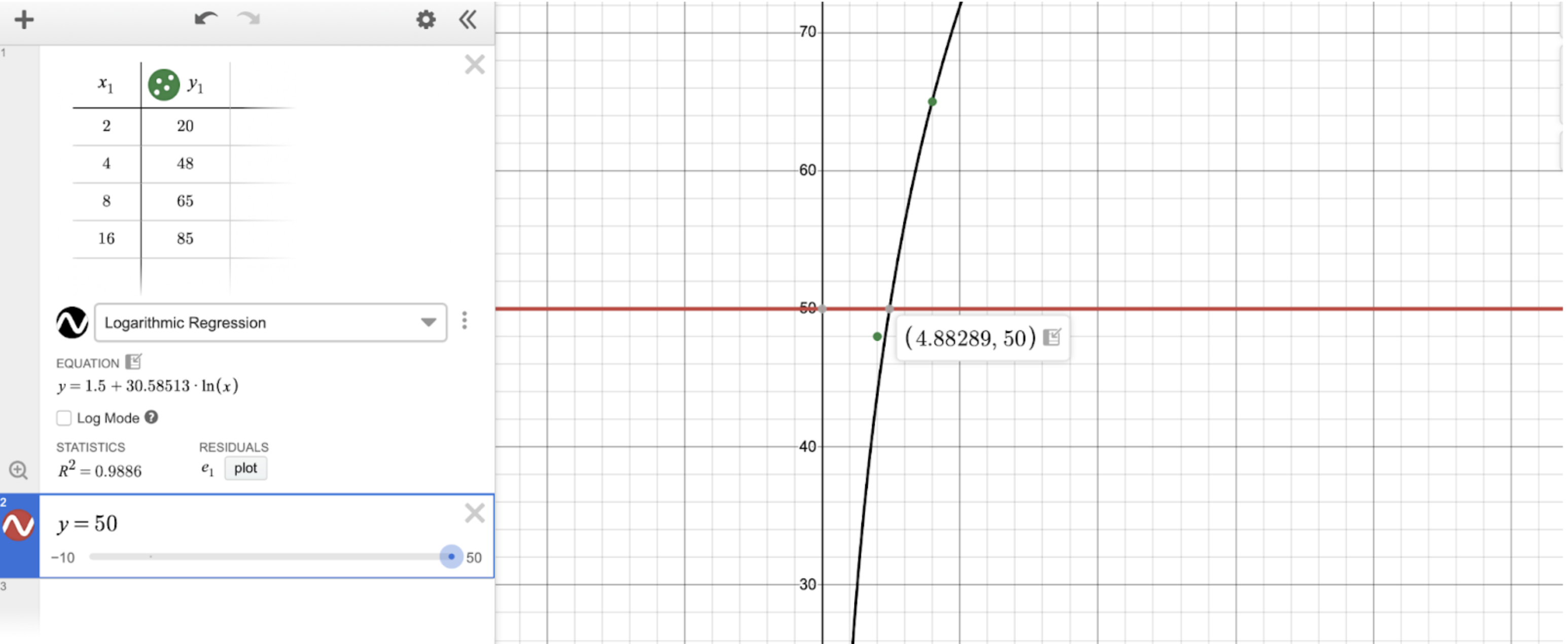
As you can see, the horizontal line at $y=50$ intersects the graph at the $x=4.88289$. For the AP exam, rounding to three decimal places, the concentration of $50mg/L$ occurs at approximately $4.883\mathrm{hours}$.

Let’s look at another situation. Suppose a biologist is studying the population of a small fish species in a pond. The population grows quickly at first but then slows as resources become limited. The biologist collects the following data:

$\begin{array}{cc}\text{Time (months) }(x)& \text{Population }(y)\\ 1& 120\\ 2& 200\\ 4& 350\\ 8& 500\end{array}$

First, we would use technology, like Desmos, to perform a logarithmic regression and find the function that best fits the data. Once the regression function is created, we can use it to make predictions about the population at times not listed in the table.

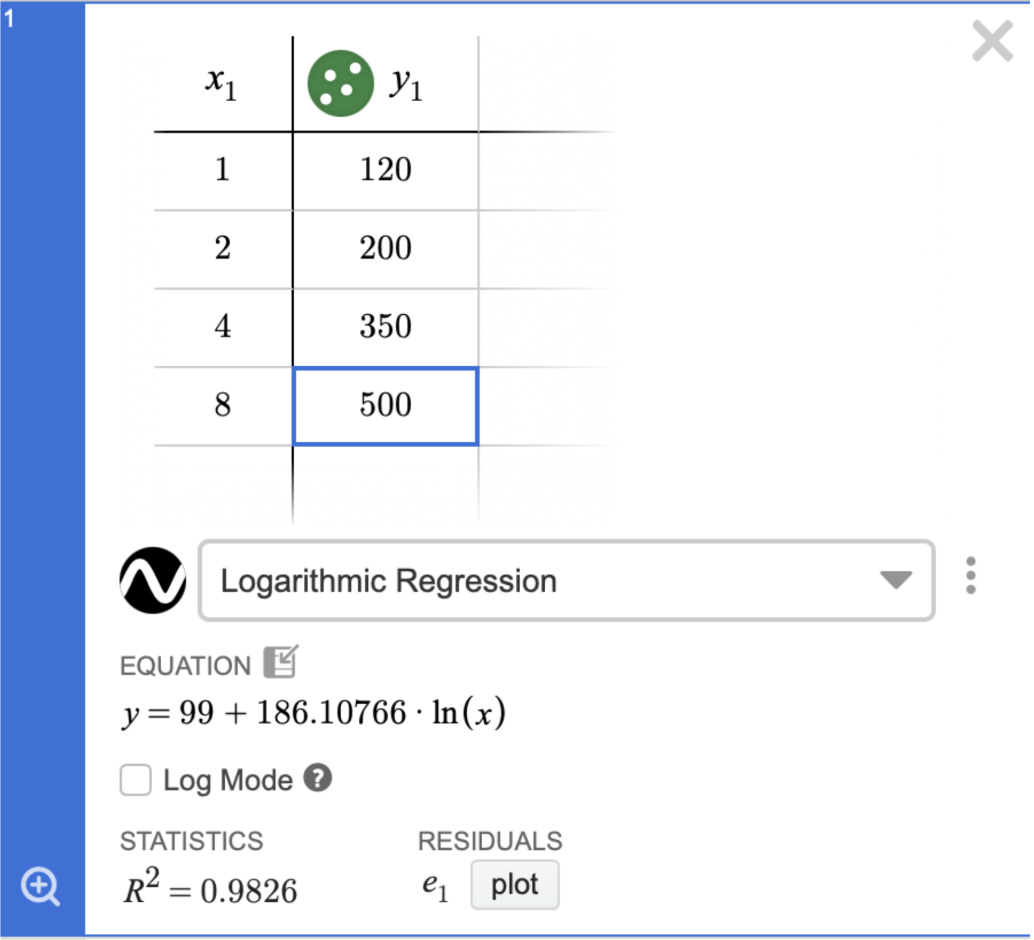
If we wanted to know the population after $5$ months, we could type $x=5$ into Desmos and, by looking at where this vertical line at $x=5$ intersects the regression graph, find the estimated population at that time.

As you can see, the vertical line at $x=5$ intersects the regression graph at the $y=398.52872$. For the AP exam, rounding to three decimal places, the estimated population of the fish after $5\mathrm{months}$ is approximately $398.529$.

Let’s say we wanted to figure out when the population reaches $450\mathrm{fish}$. We can type $y=450$ into Desmos and look at the regression graph. By seeing where the horizontal line at $y=450$ intersects the curve, we can find the $x-$value of that point, which gives the approximate number of months it takes for the population to reach $450$.

As you can see, the horizontal line at $y=450$ intersects the regression graph at $x=6.59298$. For the AP exam, rounding to three decimal places, the population reaches $450$ fish at approximately $6.593$ months.

Practice Questions

Questions

Answers to Practice Questions