Introduction

Howdy! Today we will be covering semi-log plots. This topic may seem a bit out of place in the AP Precalculus course, but regardless, it is nearly guaranteed to appear in the AP exam.

Course and Exam Description Overview

The AP Precalculus Course and Exam Description describes the following as topics you need to know for the AP Exam in May:

In these learning objectives, the AP Program expects you to recognize when to use a semi-log plot, as well as how to use semi-log plots to linearize data.

What Is a Semi-Log Plot?

A semi-log plot is defined as a plot where one of the axes is linearly scaled and the other axis is logarithmically scaled. Usually, the $y-$axis will be the axis that is logarithmically scaled. So, how does this compare to a more “typical” graph?

Well, let’s use an example graph of $\frac{1}{2}{e}^x$. The graph on a typical coordinate plane is given below.

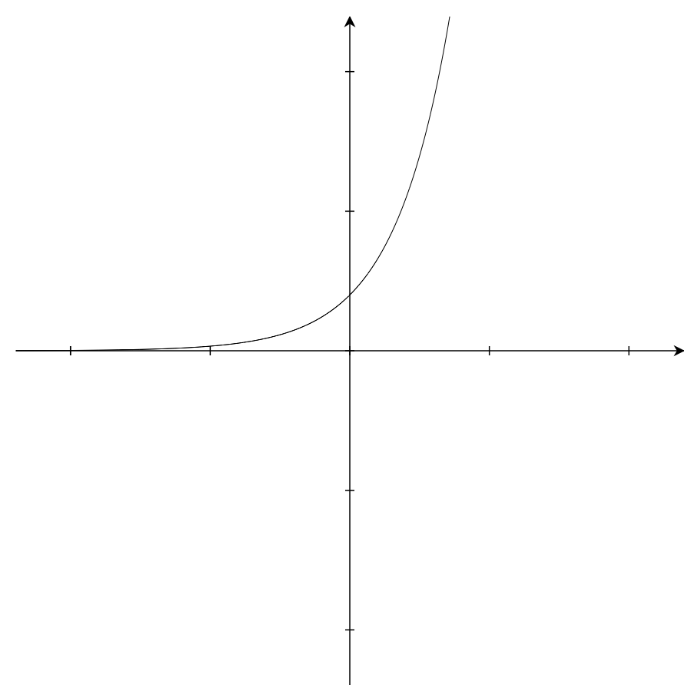
However, in a semi-log plot where the $y-$axis is logarithmically scaled, the graph of $y=\frac{1}{2}{e}^x$ looks like this. 

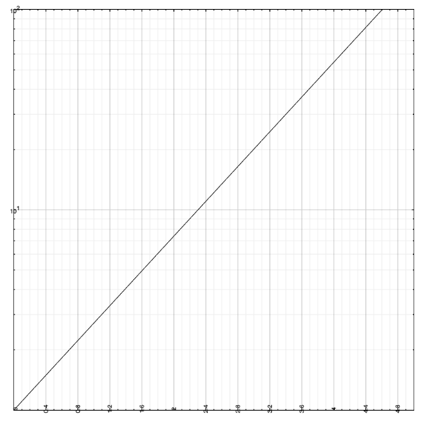
As you can see, any exponential graph will appear to be linearized on a semi-log plot.

So, what is the point of this? Well, semi-log plots are useful for graphing both extremely large and extremely small values without using an enormous amount of space. Additionally, plotting exponential data on a semi-log plot is useful when one needs to linearize data in order to make computations with said data much easier. Additionally, if you are planning to take any AP Physics course in the future, linearization of data will be an important skill to have.  

The AP exam will generally test your ability to do one of or multiple of the following:

Linearizing Exponential Data

To linearize an exponential model, we will use a semi-log plot where the $y-$axis is scaled logarithmically. For any exponential model $y=b^x$, the linearized model can be provided by $y=({\log }_{n}b)x+({\log }_{n}a)$, where $({\log }_{n}b)$ is the linearized slope, and $({\log }_{n}a)$ is the “initial value,” or the vertical axis intercept. We can use any value of $n$, but it must be greater than zero, and it cannot equal one (because $lo{g}_1(x)$ is undefined). However, you will commonly see $n$-values of $e$ (for the natural logarithm) and $10$ (for the common logarithm). 

An easy way to remember which term goes where is that the base of the function is always going to be the “slope” of the linearized model, and that the coefficient that the base is multiplied by is the “intercept” of the linearized model. 

Let’s put this into practice by doing a few problems.

Example: A data set that appears exponential is modeled by the function $f$ given by $f(x)=5\cdot 3.3^x$. The data are represented using a semi-log, where the vertical axis is logarithmically scaled with the natural logarithm. Which of the following gives the slope of the data as they appear in the semi-log plot?

Solution: Recall that for an exponential function $f(x)=a\cdot b^x$, its linearized form will be $y=({\log }_{n}b)x+{\log }_{n}a$. In this problem, our base is $3.3$, and the coefficient that the base is being multiplied by is $5$.

Therefore, our linearized form is $y=({\log }_{n}3.3)x+{\log }_{n}5$. Again, it’s up to us to use any value of $n$ we deem fit, so I’ll use $n=e$. Our final linearized form is now $y=(\ln 3.3)x+\ln 5$.

However, the question is only asking us for the slope of this linearized function. Thus, our final answer is $\ln 3.3$. 

Sometimes, you will be asked to perform the opposite, where you’re given the linearized model and are expected to find the original exponential function.

Example: A data set is represented using a semi-log plot, where the vertical axis is logarithmically scaled. On the semi-log plot, the data appear linear and can be modeled by $y=(\ln 4.1)x+\ln 6.7$. Write a function that could represent the data set on the $xy-$plane.

Solution: In this problem, we are given a linearized function in the form of $y=({\log }_{n}b)x+{\log }_{n}a$. We’ll need to convert this back into a function in the $xy-$plane, and the easiest way to do this is to convert this into an exponential function. Remember that the slope of the term with $x$ in it is the base of the exponential function, and the “intercept” is the coefficient that the base is multiplied by. Therefore, our function in the $xy$-plane is $y=6.7\cdot 4.1^x$. The base of the logarithms does not matter in this conversion to a function in the $xy-$plane.

Practice Problems