
Introduction
Linear regression models are very useful in predicting values between two variables, however, like with any prediction, there is error in its accuracy. In this topic, we will look at residuals, what they are, how to calculate them, and how to create and interpret a residual plot.
Residuals
The difference between the observed and predicted value of the response variable at a certain value of the explanatory variable is called the residual. Residuals are typically represented by either the symbol or . The formula for a residual is , or more simply residual = observed - predicted .
Residuals are not just the magnitude of the distance between the observed and predicted values, but also convey information through the sign of the residual. A positive residual means that the observed value is higher than predicted value, and that the linear regression model underpredicted the actual value. If the sign of the residual is negative, the observed value is lower than the predicted value, and so the model overpredicted the actual value.
Interpreting the meaning of a positive or negative residual is also important. On a linear regression model of test scores to study time, you would want to have a positive residual, as it means you got a higher test score than predicted for the amount of time you studied. On the other hand, for a model of insurance premiums based on age, you would want to have a negative residual, as that would mean you are paying less than expected for your age.
Residual Plots
By plotting each point on the scatterplot with the response variable as its residual, you get what’s known as a residual plot. Residual plots can be very important to understanding whether a linear regression model is appropriate for a data set.
With a true linear association between two variables, the variation between the response variable and the linear regression line will be random. Therefore, looking at a residual plot, all the points should be random and so no trend. A trend in the residual plot shows that the data is not best as a linear form and instead something non-linear.
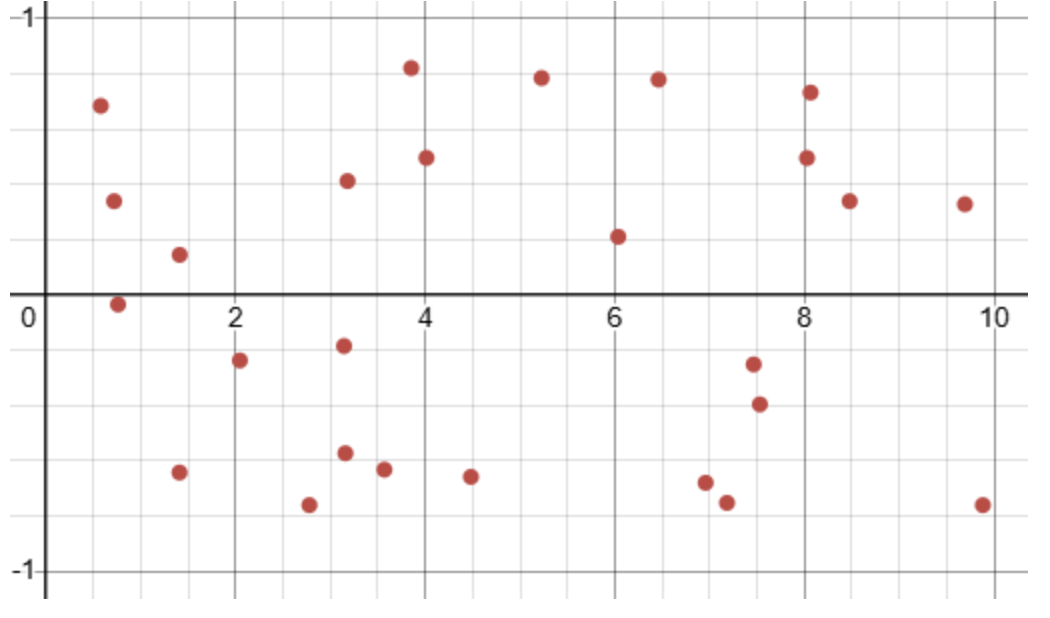
Here is an example of a residual plot. The value of residuals has no association with the explanatory variable, and so we can say that a linear association is an appropriate fit for this data set.
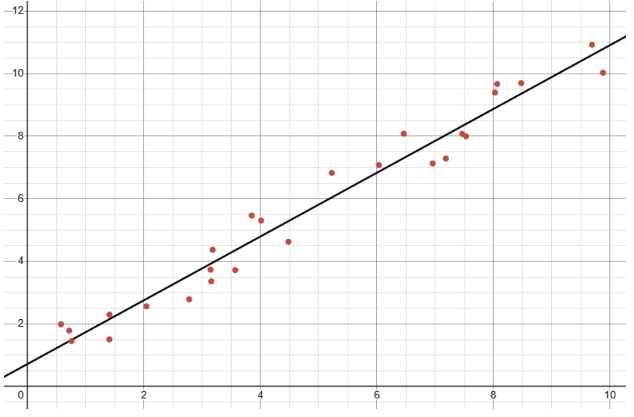
Looking at the actual scatterplot and linear regression line confirms this, as the response variable values are randomly variated around the predicted values of the linear regression model.
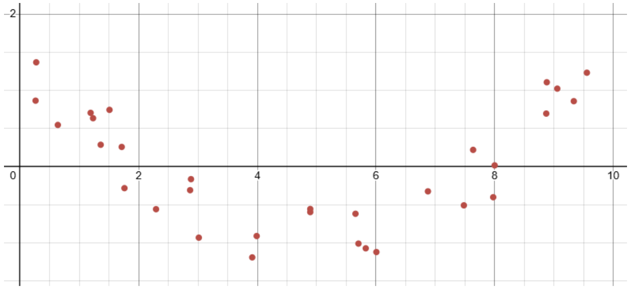
With this example , however, the residual plot shows an association between the residual and explanatory variable. This means that, even if there is a high linear correlation, a linear association is not the best fit for this data set.
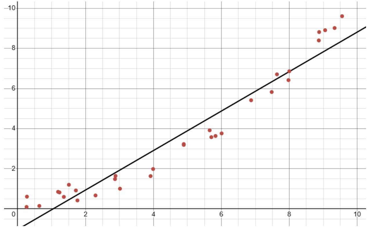
The scatterplot and linear regression line for this data set confirm these ideas. This linear regression model has a correlation coefficient of 0.968, but is clearly non-linear in form.