Introduction

Howdy! Welcome back to another AP Precalculus article. Today we will be discussing Topic 1.5 – Polynomial Functions and Complex Zeros. In topic 1.4, we covered rates of change in polynomial functions. Today, we'll be taking a look at zeros of polynomial functions, complex zeros, as well as the distinction between an even and odd function. Despite the name of the topic, this topic actually covers far more than merely complex zeros, so let's get going.

AP Course and Exam Description Overview

The AP Course and Exam Description expects you to know the following for the AP exam in May:

This topic is going to be extremely important in the multiple-choice section of the AP exam; usually at least two multiple-choice questions will appear on this topic.

Successive Differences and Degrees

The AP Course and Exam Description groups the topics above under identifying the key characteristics of a polynomial function with either suitable factorizations or with technology. Let's start off by imagining that we don't actually have a graph, but instead have just a table representing plotted values of a polynomial function $p(x)$. Shocking, I know, right?

$\begin{array}{cc}x& f(x)\\ 1& 4\\ 2& 0\\ 3& -6\\ 4& -14\\ 5& -24\end{array}$

Given such a data table, we can then see what the difference in the outputs are. We can then take the differences of said differences and keep repeating the process $n$ times, where $n$ is a positive integer. This is the process of taking an $n$th order difference. You stop at the $n$th order, where the difference is CONSTANT AND NONZERO. In other words, until the output values have a constant rate of change. In doing the process, you have thus proven that the polynomial is of degree $n$. Let's work through an example to solidify the concept:

Side note: This will ONLY work if the intervals of $x$ are equally spaced! If they are not equally spaced (i.e. you're given values of $x$ that go something like $-2,0,1,5,6,7$), this method will not work.

As you can see in the image below, we're trying to work towards the $n$th successive difference that is constant, as that is what will match the degree of the polynomial. In this case, the 2nd successive difference is constant, so our function is a second-degree polynomial, or a quadratic! :D 

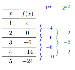
Figure 1.5.1: A table showing the second difference of $f(x)$.

Below is an example of a table which is not a second order. Given enough data, you could extend this process forever. Seeing as the fourth-order differences are nonzero and constant $(+24)$, we have thus successfully determined that the function is a fourth-degree polynomial.

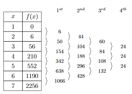
Figure 1.5.2: The fourth-order differences of polynomial $f(x)$. 

This is something that they will 100 percent ask about on the AP exam free-response questions! You will be required to determine the type of function based on a table or a graph. If the graph given to you in the FRQ is a polynomial, the scoring guidelines will require you to use a justification that is similar to this: $f$ is a quadratic function because the 2nd successive differences of the function $f$ over equal-length intervals is constant. (emphasis on the equal-length intervals and the successive differences part).

The Fundamental Theorem of Algebra

The Fundamental Theorem of Algebra states that any polynomial of a degree $n$ must have $n$ roots or zeros. A zero of a function is where the graph crosses the $x$-axis, or the linear factors of the polynomial. When written in $x$-intercept form $(x-a)(x-b)$, $a$ and $b$ are zeros.

But wait! The following graphs are of functions that only intersect the $x-$axis fewer times than their degree! So how can this be true?

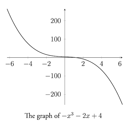
Figure 1.5.3: A graph of $-x^3-x+4$.

Well, the graph of the function above has either zeros with more than one multiplicity (i.e., they "repeat" or exist more than once). Other functions may have zeros that are something called imaginary or complex zeros.  That is, they do not actually exist on the $xy-$ plane, but they do exist due to the Fundamental Theorem of Algebra. 

Even and Odd Functions

Functions can have two types of symmetry: rotational symmetry and $y-$axis symmetry. Functions with these types of symmetry can be classed as odd or even functions respectively. Of course, other functions can have no symmetry; however, we will focus on functions which do have symmetry. 

Rotational or origin symmetry is a type of symmetry where functions have symmetry about the origin. These functions are also known as odd functions because of something we'll see in a moment. Functions with rotational symmetry satisfy the condition $f(-x)=-f(x)$. This means that for each point $(x,y)$ that exists for the function in the coordinate plane, there must be a point $(-x,-y)$ where the function is also defined. Another way to think about this is that the function, when reflected over the $y$-axis, is identical to its $x$-axis reflection. The following graph shows an example of a function with rotational symmetry.

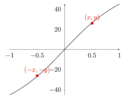
Figure 1.5.4: A graph of a polynomial function possessing rotational symmetry.

$y-$axis symmetry is another type of symmetry where functions have symmetry about the $y-$axis. These functions are known as even functions. Functions with $y$-axis symmetry satisfy the condition $f(-x)=f(x)$. That is, for each point $(x,y)$ that exists for the function in the coordinate plane, there must be a point $(-x,y)$ where the function is also defined. In other words, reflecting the function about the $y$-axis does not change the function. The following graph shows an example of a function with $y-$axis symmetry.

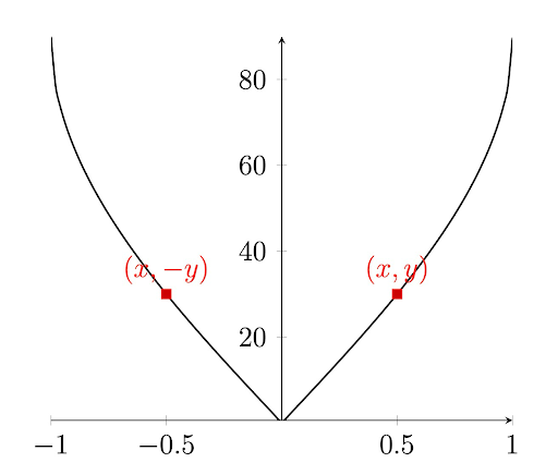
Figure 1.5.5: A graph of a polynomial function possessing $y-$axis symmetry. 

Specifically for polynomials, any polynomial with an odd degree and is centered about the origin is going to have rotational symmetry, while any polynomial raised to an even degree and is centered about the $y-$axis is going to have $y-$axis symmetry. This is an easy way to remember what an odd function is: odd polynomials are raised to an odd degree, and even polynomials are raised to an even degree.

Zeros and Multiplicity

One of the reasons why a function might actually have fewer $x–$intercepts than zeros is because of zeros with multiplicity. Multiplicity defines the number of times that a zero $x=a$ exists for a function. Let's take a look at the graph of the function $f(x)=x^3-3x^2+4$.

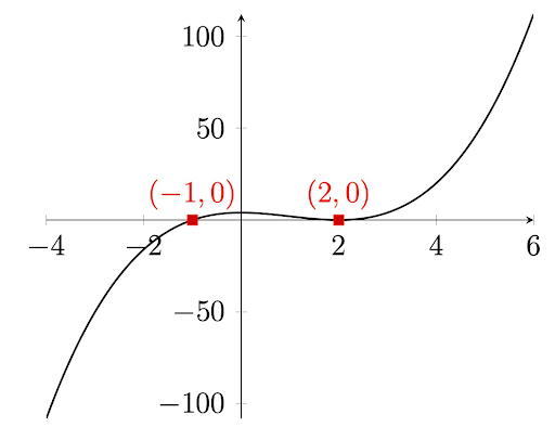
Figure 1.5.6: A graph of a polynomial function with roots at $(-1,0)$ and $(2,0)$.

If we were to evaluate the zeros of this function, we would get $f(x)=(x+1)(x-2{)}^2$, which is the graph written in intercept form. Let's pause here for a moment. The function has three zeros, and it is raised to the third degree. Therefore, it satisfies the Fundamental Theorem of Algebra.

But you'll notice that there are only two $x-$intercepts. Why is that? It's because one of the zeros, $x=2$, actually has a multiplicity of $2$. You'll also notice that at this zero, the function "bounces" back up; for zeros of a multiplicity of $1$, the function will always pierce through the $x-$axis.

Let's now take a look at the graph of the function $f(x)=x^5+3x^4-46x^3-146x^2-147x-49$.

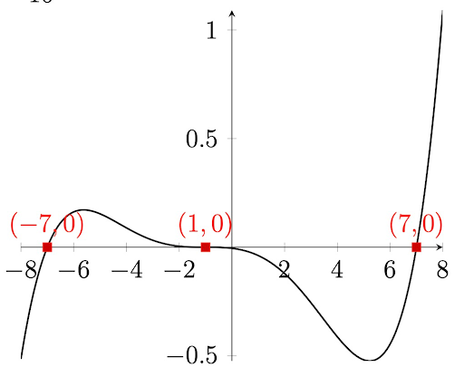
Figure 1.5.7: A graph of function $f(x)=x^5+3x^4-46x^3-146x^2-147x-49$. 

But wait! The polynomial is raised to a fifth degree and there's only three graphed zeros! If we were to factor this function, we would get $f(x)=(x+7)(x+1{)}^3(x-7)$. We can see that one of the linear factors, $x+1$, has a multiplicity of $3$.

From here, we can see a trend: The multiplicity dictates the function behavior at that zero. Where a function has a real zero with an even multiplicity, the function will just "bounce off" the zero. Where a function has a real zero with an odd multiplicity greater than $1$, the function will "level out" such that the slope of the function at the zero is, well, zero.

In other words, any sign change undergone by a function ALWAYS goes through a linear factor of odd multiplicity. Any bounce undergone by a function ALWAYS goes through a linear factor of even multiplicity, with the graph being tangent to the $x$-axis at that point.

This can be used to more easily solve polynomial inequalities, as we now know that if the function is positive for a value of $x$ not that much smaller than the zero with an even multiplicity, the function is also positive for a value of $x$ not that much larger than the zero with an even multiplicity.

For example, let's say that we want to find all values of $x$ for which the function $p(x)=\frac{1}{4}(x)(x+2)(x-4{)}^2$ is greater than $0$. The first thing to do is to construct a sign chart, which is a glorified number line marking where the function is equal to $0$. Here, we label the zeros of the functions as they are the points where the graph can change from positive and negative.

Figure 1.5.8: Constructing a sign chart. 

Next, we'll test values of $x$ in between the zeros of $x$ but with a catch: we only need to find the value of one point. We can figure out the rest of the ranges with multiplicities. If an even multiplicity zero separates two ranges, the sign is the same. If the zero is odd, the two ranges will have opposite signs. Check out sample values below to see what I mean.

Figure 1.5.9: Placing values on the sign chart. 

Therefore, we know that $p(x)$ is greater than $0$ on the interval $(0,4)$ and $(4,\infty )$. Remember that at the zeros of $p(x)$, $p(x)=0$, and is therefore not greater than $0$. 

Note: You don’t actually need to calculate the numerical values. Just figure out whether a range is positive or negative, and logically build the rest of the ranges with multiplicity rules. You can pull all positive or negative ranges as the answer depending on whether the problem is asking for.

Complex Zeros

While the multiplicity of real zeros can help us satisfy the Fundamental Theorem of Algebra, it will not always satisfy an important condition: the degree of the polynomial matches the number of zeros that a polynomial has. There are, however, complex or imaginary zeros. These zeros are zeros that do not exist in the $xy-$plane, but exist to satisfy the Fundamental Theorem of Algebra.

Non-real zeros of a polynomial always exist in conjugate pairs, or as siblings effectively. That's to say, if $a+bi$ is an imaginary zero of a polynomial function $p$, then $a-bi$ is also a zero of $p$, where $a$ and $b$ are constants. $i$ is the imaginary component and refers to $\sqrt{-1}$. (When referring to a conjugate, the term $bi$ is what is changing sign; the real term $a$ does not change signs.)

Example: A function $p(x)$ is raised to the fourth degree and has the real zeros $x=-3$, $x=4$, and the imaginary zero $x=2+2\sqrt{2}i$. Find the remaining zeros of $p$.

Since our polynomial is raised to the fourth degree, we know that we have four total zeros. We have two real zeros and an imaginary zero, so we've already identified three of them. Remembering that complex zeros exist in conjugates, we can deduce that the other zero must be imaginary, which is $x=2-2\sqrt{2}i$.

Practice Questions