INTRODUCTION

Howdy! Today we will be going over rational functions and their end behavior. We already covered the basics of end behavior, as well as how to use limit notation, in topic 1.6. Therefore, I will be including a brief recap of end behavior, but if you need a more comprehensive overview of end behavior and how to use limit notation to express end behavior, I recommend referring to the article on topic 1.6 of AP Precalculus.

COURSE AND EXAM DESCRIPTION BREAKDOWN

The AP Precalculus Course and Exam Description (CED) states that you need to know the following for the AP Exam:

If the leading term of the polynomial in the denominator has a greater degree than the leading term of the polynomial in the numerator, the rational function’s horizontal asymptote is expressed as $y = 0$ . Describing end behaviors of rational functions based on the leading terms of each polynomial. (We’ll discuss what this means in a moment.)
If the leading term of the polynomials in the numerator and in the denominator are of the same degree, the rational function’s horizontal asymptote is expressed as $y = \frac{a}{b}$ , where $a$ is the coefficient of the leading term of the polynomial in the numerator, and $b$ is the coefficient of the leading term of the polynomial in the denominator.
If the leading term of the polynomial in the numerator has a greater degree than the leading term of the polynomial in the denominator, the rational function has an oblique asymptote. This oblique asymptote will have a non-zero slope with the end behavior either indicating that the rational function either increases or decreases without bound based on whether its input is increasing or decreasing without bound.

BASICS OF RATIONAL FUNCTIONS

A rational function is any function where a polynomial is divided by a polynomial, or a quotient of two rational functions. Generally, rational functions are written in the form $r (x) = \frac{p ( x )}{q ( x )}$ , where $p (x)$ and $q (x)$ are polynomial functions (including reduced polynomials like quadratics and lines).

A NOTE ON END BEHAVIOR ASYMPTOTES

In many elementary algebra courses, an asymptote is defined as a line that a curve gets really close to but never touches. This is not always the case. Rational functions can in fact cross their horizontal, slant, or oblique asymptotes. This is extremely important because you will be asked to find these crossing points on the AP Exam. However, we will discuss that in another article. So, why mention this at all? . . .

A rational function’s horizontal, slant, or oblique asymptote is more generally referred to as an end behavior asymptote. This allows us to not only be more general as to what we are looking for when finding these types of asymptotes, which is the end behavior of the rational function, but also to establish that these asymptotes are not lines that a rational function may never cross.

One more note: The property of a rational function being able to cross an asymptote ONLY applies to end behavior asymptotes. A rational function may NEVER EVER cross one of its vertical asymptotes. If you find that a rational function does cross one of its vertical asymptotes, you need to check your work somewhere.

EVALUATING THE END BEHAVIOR OF RATIONAL FUNCTIONS ALGEBRAICALLY

Just like when we evaluated the end behavior of polynomial functions, we will be focusing on the leading terms of each polynomial; the subsequent terms with lower degrees are guided by the leading term when it comes to end behavior. However, we will use these leading terms a bit differently to evaluate the end behavior of a rational function; instead of looking at either leading term independently, we will be looking at the relation between both leading terms.

As a clarification, the leading term is NOT the first term of the polynomial! The leading term is the term that is raised to the highest power. This is a very important distinction to keep in mind.

In this case, we will be taking a look at three situations:

When the degree of the leading term of the polynomial in the denominator is greater than the degree of the leading term of the polynomial in the numerator.
When the degree of the leading term of the polynomial in the denominator is the same as the degree of the leading term of the polynomial in the numerator.
When the degree of the leading term of the polynomial in the numerator is greater than the degree of the leading term of the polynomial in the denominator.

Degree of the Leading Term of the Polynomial in the Denominator is Greater than the Degree of the Leading Term of the Polynomial in the Numerator

When the leading term of a polynomial in the denominator is raised to a power greater than the leading term of a polynomial in the denominator, the rational function will approach zero as its input either increases or decreases without bound. This can be expressed in two ways: either indicating that its horizontal asymptote is the line $y = 0$ or expressing the end behavior as a limit. 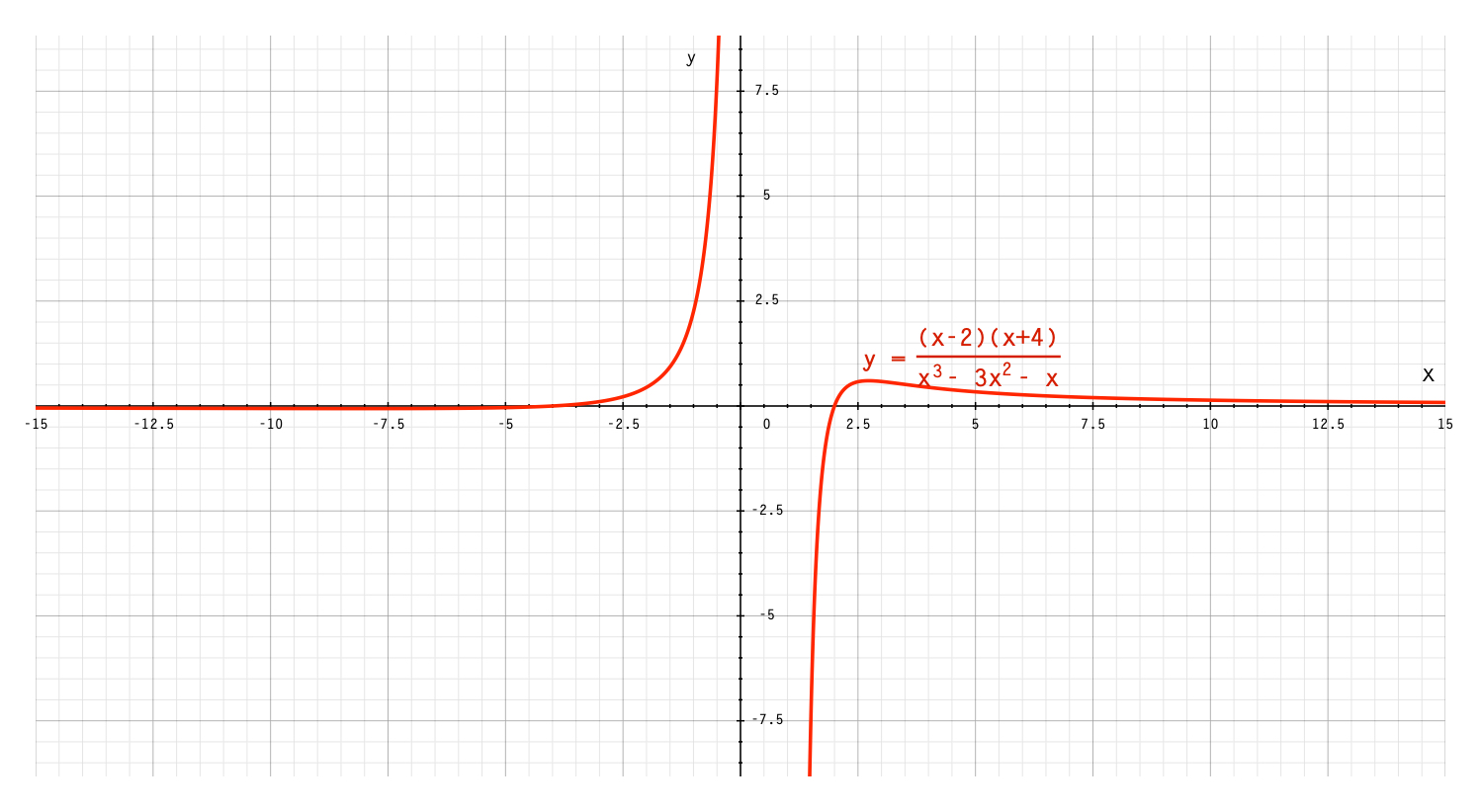In this case, the end behavior will be expressed as $x \to \infty lim r (x) = 0$ and $x \to - \infty lim r (x) = 0$ .

Example 1: Evaluate the end behavior of the function $r (x) = \frac{( x - 2 ) ( x + 4 )}{x ^{3} - 2 x ^{2} + x}$ as $x$ increases without bound and as $x$ decreases without bound.

Solution 1: We will start by identifying the degree of the leading term of the polynomial in the numerator and in the denominator. For the polynomial in the denominator, it is easy; our leading term is $x^{3}$ , which is raised to the third degree. The leading term of the numerator is not so obvious at first due to it being factored. We can, however, see that there are two factors, which indicates that the denominator’s leading coefficient is raised to the second power; to verify, if we were to expand the numerator, we would end up with $x^{2} + 2 x - 8$ .

Because the degree of the leading term of the denominator is greater than the degree of the leading term of the denominator, our rational function is going to approach 0 as its input $x$ increases or decreases without bound. We can express this in limit notation as $x \to - \infty lim = 0$ and $x \to \infty lim = 0$ .

I’ll also provide a graph of the rational function $r (x)$ below to demonstrate what this means graphically. Additionally, you will see an example of what I mean when the rational function crosses its horizontal asymptote.

As you can see from the graph, the function approaches the horizontal line $y = 0$ as its input increases/decreases without bound.

Degree of the Leading Term of the Polynomial in the Numerator and the Degree of the Leading Term of the Polynomial in the Denominator are the Same

When the leading term of the polynomial in the numerator of a rational function and the leading term of the polynomial in its denominator are raised to the same degree, the end behavior can be expressed as a horizontal asymptote $y = \frac{a}{b}$ , where $a$ is the coefficient of the leading term of the polynomial in the numerator and $b$ is the coefficient of the leading term of the polynomial in the denominator. If we were to express this in limit notation, as the rational function’s input $x$ increases without bound, $x \to \infty lim r (x) = \frac{a}{b}$ , and as $x$ decreases without bound, $x \to - \infty lim r (x) = \frac{a}{b}$ .

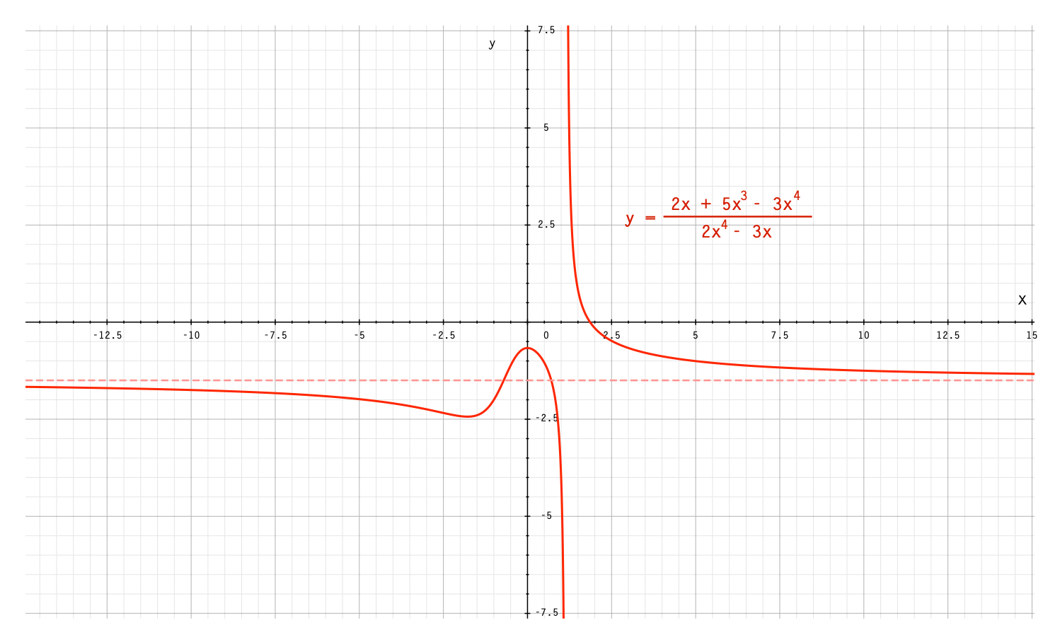
Example 2: Evaluate the end behavior of the rational function $r (x) = \frac{2 x + 5 x ^{3} - 3 x ^{4}}{2 x ^{4} - 3 x} a s$ @x$ increases without bound and as $x$ decreases without bound.

Solution 2: Just like the previous example, we will identify the leading terms of the polynomials in the numerator and denominator. Note that for the polynomial in the numerator, the leading term is NOT $2 x$ . Even though it appears first, it is not the term raised to the highest power, which is $- 3 x^{4}$ . For the polynomial in the denominator, the leading term is $2x^4$. Because the degree of these leading terms is the same, we will divide the coefficients to get our horizontal asymptote, which is $y = \frac{- 3}{2}$ . If we were to express this in limit notation, as the rational function’s input $x$ increases without bound, $x \to \infty lim r (x) = \frac{- 3}{2}$ , and as $x$ decreases without bound, $x \to - \infty lim r (x) = \frac{- 3}{2}$ . A graphical representation of the function is located below.

Degree of the Leading Term of the Polynomial in the Numerator is Greater than the Degree of the Leading Term of the Polynomial in the Denominator

When the leading term of the polynomial in the numerator is raised to a higher power than the leading term of the polynomial in the denominator, the rational function has no horizontal asymptote, and as such, the function will not approach a constant value. Instead, it will either approach positive or negative infinity. So, how do we figure out the end behavior of the rational function as its input increases or decreases without bound? We will need to perform polynomial long division, where we will divide the polynomial in the numerator by the polynomial in the numerator. This will allow us to find its oblique asymptote.

Side note: Why do I not call these oblique asymptotes a slant asymptote? The reason is because not all asymptotes of this type of rational function are slant asymptotes. A slant asymptote indicates that the asymptote is linear with a nonzero slope. As you will soon see, not all rational functions have slant asymptotes; they may have asymptotes in the shape of polynomials raised to a higher degree. A slant asymptote, however, is a type of oblique asymptote, and thus I will collectively refer to asymptotes of this type of rational function as slant asymptotes.

Example 3: Evaluate the end behavior as $x$ increases without bound and as $x$ decreases without bound of $t (x) = \frac{6 x ^{3} + 3 x - 12}{3 x ^{2} - 3 x}$ using the mathematical expression of a limit.

Solution 3: Because the polynomial in the numerator is raised to a higher degree than the polynomial in the denominator, we will need to perform polynomial long division to find the slant asymptote. The procedure to perform polynomial long division looks like this:

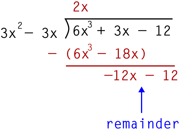
As a general refresher for polynomial long division, you will divide the first term of the dividend (the polynomial inside the braces) by the first term in the divisor (the polynomial to the left of the braces). The result of that will form part of the quotient (above the braces). Then, you will multiply that term in the quotient by the second term in the divisor and subtract that from the dividend. Then, you will rinse and repeat until you reach a term in the dividend that you are not able to divide by the first term of the divisor. That will be your remainder, which does not matter much for the oblique asymptote; we only care about the quotient. As you can see, our quotient is $2 x$ , which is our slant asymptote. However, we are not done; the problem asked us to express the end behavior using the mathematical expression of a limit. That is fairly simple; we just need to evaluate the end behavior of the leading term of the asymptote. Because this is a line with positive slope, as $x$ increases without bound, $x \to - \infty lim t (x) = - \infty$ and $x \to \infty lim t (x) = \infty$ . Let’s go ahead and graph this rational function to see this in action.

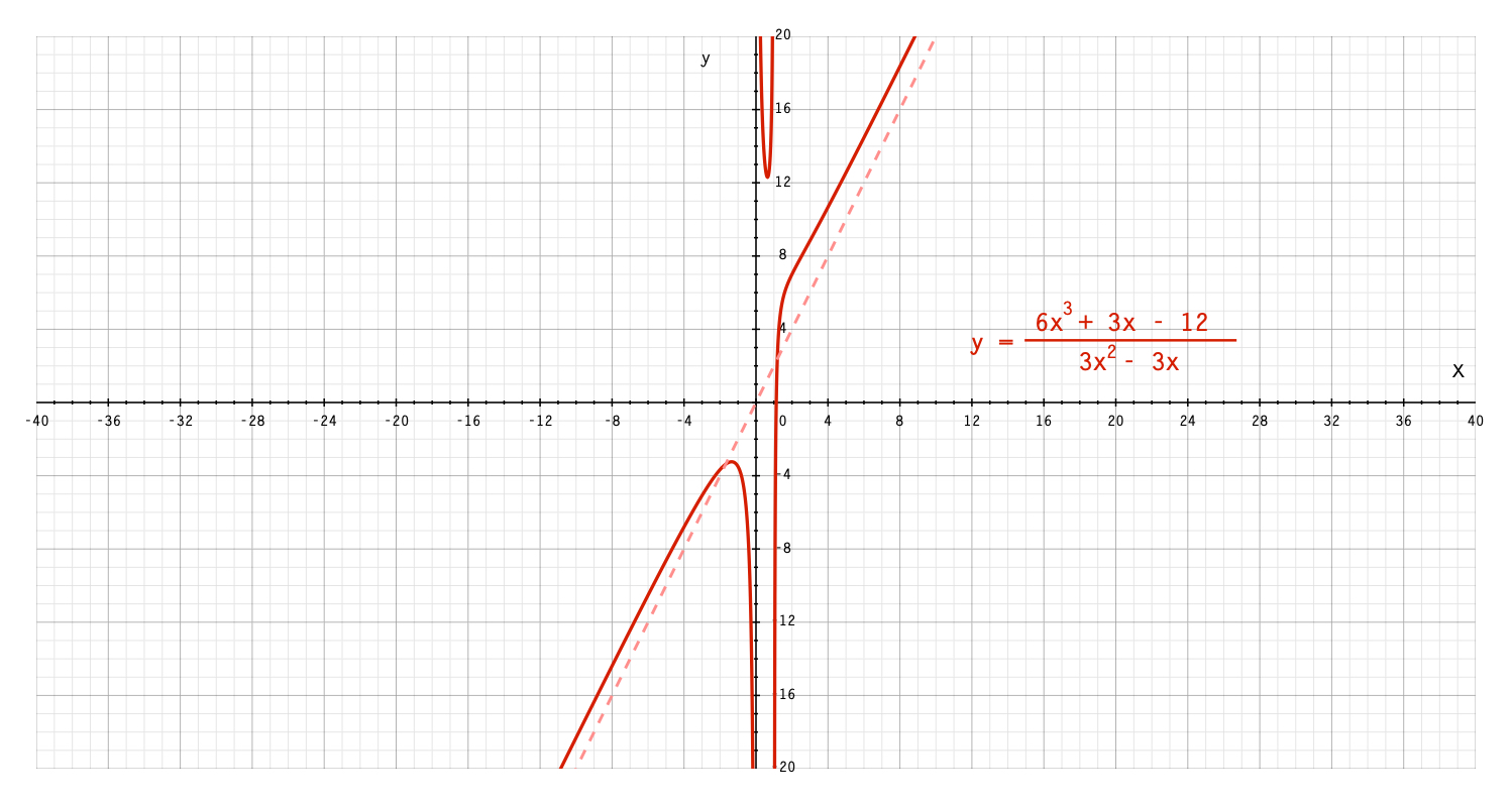
While it may not be so obvious in the graph shown above, the rational function “wraps” around the end behavior asymptote $y = 2 x$ . Additionally, you can see how the graph of the rational function increases without bound as its input increases without bound, and decreases without bound as its input decreases without bound.

THE ACRONYM, FINALLY!

So, how can we remember all of this? Well, we can use an acronym that many of you may be familiar with: BOBO BOTNA EATS DC.

BOBO stands for bigger on bottom = 0. This means that the horizontal asymptote will be $y = 0$ ; if we were to think about this in limit notation, as the limit as the input of the rational function increases or decreases without bound, the output of the rational function will approach zero.

BOTN stands for bigger on top; no [horizontal asymptote]. This means that the end behavior asymptote will be a slant or oblique asymptote, and you will need to perform polynomial long division to find the asymptote or evaluate the end behavior of the rational function.

EATS DC stands for exponents are the same; divide coefficients. This means that if the degree of the leading term of the polynomial in both the numerator and the denominator are the same, you merely divide the coefficients to find the asymptote. For a rational function $r (x)$ , if we let $a$ be the coefficient of the leading term of the polynomial in the numerator and $b$ be the coefficient of the leading term in the denominator, the horizontal asymptote will be $y = \frac{a}{b}$ . Additionally, the end behavior as the input $x$ of the rational function either increases or decreases without bound can be expressed as $x \to - \infty lim r (x) = \frac{a}{b}$ and $x \to \infty lim r (x) = \frac{a}{b}$ .

And there you have it! You now know how to evaluate the end behavior of rational functions. Stay tuned for the article on topic 1.8, which will be about how to find the zeroes of rational functions.

PRACTICE PROBLEMS ON AP PRECALCULUS TOPIC 1.7

Problems 1-5: For these problems, write a rational function that satisfies the given conditions.

$x \to - \infty lim r (x) = 0$ and $x \to \infty lim r (x) = 0$
$x \to - \infty lim s (x) = \frac{5}{7}$ and $x \to \infty lim r (x) = \frac{5}{7}$
$x \to - \infty lim t (x) = - 3$ and $x \to \infty lim r (x) = 3$
$x \to - \infty lim u (x) = - \infty$ and $x \to \infty lim r (x) = \infty$
$x \to - \infty lim v (x) = \infty$ and $x \to \infty lim r (x) = - \infty$

Problems 6-8: For these problems, evaluate the end behavior of the given rational function algebraically as $x$ increases without bound and as $x$ decreases without bound. Express your answers using the mathematical expression of a limit.

$r (x) = \frac{3 x - 4 x ^{3} + x}{9 x ^{2} + 4 x ^{3} - x ^{5}}$
$t (x) = \frac{6 x ^{2} - 4 x + 1}{- 6 x + 3 x ^{2} + 9}$
$u (x) = \frac{2 x ^{4} + 8 x ^{2} - x}{( x - 3 ) ( x - 6 )}$

Problems 9-10:

Answer Guide

For Problems 1-5, the following is a guide on what your answer should satisfy as well as examples of correct answers. I recommend that you graph your answers on a graphing calculator to check your work.

$r (x)$ should have a polynomial in the numerator whose leading term is raised to a lower degree than the leading term of the polynomial in the numerator. An example of this would be $r (x) = \frac{( x + 3 ) ( x - 2 ) ( x + 5 )}{x ^{4} + 2 x ^{2} - x}$ .
$s (x)$ should have polynomials in the numerator and denominator whose leading terms are raised to the same power. Additionally, the quotient of the coefficients of the leading term of the polynomial in the numerator and the leading term of the polynomial in the denominator should be equal to $\frac{5}{7}$ . An example of this would be $s (x) = \frac{5 x ^{3} - 2 x}{7 x ^{3} - 4 x ^{2} + 1}$ .
$t (x)$ should also have polynomials in the numerator and denominator whose leading terms are raised to the same power. Additionally, the quotient of the coefficients of the leading term of the polynomial in the numerator and the leading term of the polynomial in the denominator should be equal to $3$ . An example of this would be $t (x) = \frac{3 x ^{2} - 6 x + 9}{x ^{2} + 2 x + 4}$ .
$u (x)$ should have a polynomial in the numerator raised to a degree higher than the polynomial in the denominator. Additionally, the resulting end behavior asymptote should have an end behavior such that as $x$ increases without bound, the asymptote increases without bound, and as $x$ decreases without bound, the asymptote decreases without bound. An example of this would be $u (x) = \frac{x ^{3} + 2 x ^{2} - x}{( x + 4 ) ( x + 5 )}$ .
$v (x)$ should have a polynomial in the numerator raised to a degree higher than the polynomial in the denominator. Additionally, the resulting end behavior asymptote should have an end behavior such that as $x$ increases without bound, the asymptote decreases without bound, and as $x$ decreases without bound, the asymptote increases without bound. An example of this would be $v (x) = \frac{- 4 x ( x ^{2} - x )}{( x + 4 ) ( x - 2 )}$ .
The leading term of the polynomial in the denominator is raised to a higher degree than the leading term of the polynomial in the numerator. As such, we know that as $x$ increases or decreases without bound, $r (x)$ will approach $0$ . Therefore, $x \to - \infty lim r (x) = 0$ and $x \to \infty lim r (x) = 0$ .
The leading terms of the polynomials in both the numerator and the denominator are raised to the same degree, and thus we will divide the coefficients of these leading terms to get the end behavior of the function. By doing so, we find that as $x$ increases or decreases without bound, $r (x)$ will approach $2$ . Therefore, $x \to - \infty lim r (x) = 2$ and $x \to \infty lim r (x) = 2$ .
The leading term of the polynomial in the numerator is raised to a higher degree than the leading term of the polynomial in the denominator. Therefore, we will need to perform polynomial long division first in order to find the end behavior asymptote, which is $2 x^{2} - 18 x + 134$ . Now, we will evaluate the end behavior of this asymptote; for this, we will use the skills from topic 1.6. We find that as $x$ either decreases or increases without bound, the asymptote will approach positive infinity. Since the rational function “wraps” around this end behavior asymptote as $x$ increases or decreases without bound, the end behavior of the rational function is effectively the same as that of the asymptote. Therefore, $x \to - \infty lim u (x) = \infty$ and $x \to \infty lim r (x) = \infty$ .

FiveHive