AP Precalculus Unit 2 Cram Guide

Topic 2.1 - Changes in Arithmetic and Geometric Sequences

Sequences are like functions, but only non-negative whole numbers can be plugged into them.
- The graph of sequences are dots instead of curves
There are two types of sequences: arithmetic and geometric
Arithmetic:
- Arithmetic sequences have a common difference between consecutive/successive terms.
- The difference between the second and first term of an arithmetic sequence will be the same as the difference between the third and second term of an arithmetic sequence.
- Arithmetic sequences are represented as $a_{n} = a_{0} + d n$ , where $a_{0}$ is the zeroth, or initial term, and $a_{n}$ is the $n$ -th term, and $d$ represents the common difference.
- Compare any two terms in a sequence using $a_{n} = a_{k} + d (n - k)$ , where $a_{k}$ and $a_{n}$ are two different terms of the sequence.
Geometric:
- Geometric sequences have a common ratio rather than a common difference.
- The ratio between the second and first term of a geometric sequence will be the same as the ratio between the third and second term of a geometric sequence.
- Geometric sequences are represented as $g_{n} = g_{0} r^{n}$ , where $g_{0}$ is the zeroth, or initial term, and $g_{n}$ is the $n$ -th term, and $r$ represents the common ratio.
- Compare any two terms in a sequence using $g_{n} = g_{k} \cdot r^{(n - k)}$ , where $g_{n}$ and $g_{k}$ are two different terms of the sequence.
Arithmetic and geometric sequences change in different ways.
- An arithmetic sequence may look like this: $5$ , $10$ , $15$ , $20$ .
- A geometric sequence may look like this: $2$ , $4$ , $8$ , $16$ , $32$ .
- Importance: Arithmetic sequences change equally with each step, but geometric sequences change proportionally with each step.

Topic 2.2 - Changes in Linear and Exponential Functions

Arithmetic sequences can be represented as linear functions, and geometric sequences can be represented as exponential functions.
- This extends sequences to a domain of all real numbers using functions.
Linear Functions:
- Linear functions are represented as $f (x) = m x + b$ .
  - Similar in form to $a_{n} = a_{0} + d n$ . $a_{0}$ and $b$ work the same way as an initial value, and $m$ and $d$ work the same way as a common difference or slope.
- To compare two points on a linear function, use $f (x) = y_{i} + m (x - x_{i})$
  - Similar in form to $a_{n} = a_{k} + d (n - k)$ . $y_{i}$ and $a_{k}$ work the same way, and $(n - k)$ with $(x - x_{i})$ work the same way.
- Both linear functions and arithmetic sequences are based on addition and a constant change of value.
Exponential Functions:
- Exponential functions are represented as $f (x) = a b^{x}$ . The value of $b$ cannot be $0$ or $1$
  - Similar in form to $g_{0} r^{n}$ , as $a$ and $g_{0}$ both represent initial value and $r$ and $b$ represent the common ratio.
- To compare two points on an exponential function, use $f (x) = y_{1} b^{(x - x_{i})}$
  - Similar in form to $g_{n} = g_{k} r^{(n - k)}$ . $g_{k}$ and $y_{1}$ are similar in function, and $(x - x_{i})$ and $(n - k)$ work the same way.
- Both exponential functions and geometric sequences are based on multiplication.
Identify linear and exponential functions by looking at equal-length input-value intervals. Compare the difference of the function over the same length.
- From $f (5)$ to $f (3)$ and $f (3)$ to $f (1)$ , we can compare the difference between these two.
  - If the difference between $f (5)$ and $f (3)$ is the same as the difference between $f (3)$ and $f (1)$ , the function is linear.
  - If they change proportionally $(\frac{f ( 5 )}{f ( 3 )} = \frac{f ( 3 )}{f ( 1 )})$ , then the function is exponential.

Topic 2.3 - Exponential Functions

Exponential functions have the general form of $f (x) = a b^{x}$ .
- The initial value, or $y$ -intercept, is $a$ , and the base is $b$ . The value of $a$ cannot be zero, and the value of $b$ cannot be negative or one.
- The domain of an exponential function is all real numbers.
The output values of exponential functions are proportional for equal-length input-value intervals.
- Exponential functions are always either increasing or decreasing, meaning that they have no local extrema.
- Exponential functions are either always concave up or down, meaning that they have no inflection points.
If the output values of an exponential function are not proportional over equal-length input-values, the function is shifted up or down.
Exponential functions have two different behaviors:
- If $a > 0$ and $b > 1$ , then the function demonstrates exponential growth. This means that the function increases in value as $x$ increases.
- If $a > 0$ and $0 < b < 1$ , then the function demonstrates exponential decay. This means that the function decreases in value as $x$ increases.

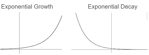
The end behavior of exponential functions can either be infinity, negative infinity, or zero. The following table shows how different conditions lead to different end behaviors.

$The values of a and b in f (x) = a b^{x} are \dots a > 0, b > 1 a > 0, 0 < b < 1 a < 0, b > 1 a < 0, 0 < b < 1 As x increases without bound \dots x \to \infty lim f (x) = \infty x \to \infty lim f (x) = 0 x \to \infty lim f (x) = - \infty x \to \infty lim f (x) = 0 As x decreases without bound \dots x \to - \infty lim f (x) = 0 x \to - \infty lim f (x) = \infty x \to - \infty lim f (x) = 0 x \to - \infty lim f (x) = - \infty$

Topic 2.4 - Exponential Function Manipulation

Product Property:
- $b^{m} \cdot b^{n} = b^{m + n}$
- Identical to a horizontal translation of an exponential function.
  - Implies that a horizontal translation is the same as a vertical dilation.
  - If $f (x) = b^{x}$ , $f (x + k) = b^{(x + k)} = b^{k} b^{x} = b^{k} \cdot f (x)$ .
Power Property:
$(b^{m})^{n} = b^{mn}$ .
Identical to a horizontal dilation of an exponential function.
- If $f (x) = b^{x}$ , then $f (a x) = b^{a x} = (b^{a})^{x}$ .
Negative exponent property:
$b^{- n} = \frac{1}{b ^{n}}$
This changes the negative exponent into a fraction with a positive exponent.
Fractional exponent to a root:
$b^{\frac{1}{k}} = k b$
- For example, $8^{\frac{1}{3}}$ is the same as the third root of $8$ $38 = 2$

Topic 2.5 - Exponential Function Context and Data Modeling

Exponential models can be constructed based on the context.
- $b$ is seen as a growth factor or a percent change.
- For example, a word problem can state that a bank account has a $2%$ interest every year beginning with $50, 000$ dollars.
  - The $2%$ interest implies that the base is $b = 1.02$ , since every year results in a $2%$ increase.
  - The initial value is $a = 50000$ . Therefore, the function is $f (x) = 50000 \cdot (1.02)^{x}$ .
  - In many contexts, the base will be the natural base $e$ , which is around $2.718$ .
Domain restrictions can be established based on the context.
- For example, an exponential function based on time cannot have $t = - 4$ because that would be negative time.
  - The domain restriction for such would not include negative inputs.
An exponential function’s unit of time may be changed depending on the question.
- For example, the function $g (d) = 500 \cdot 1. 5^{d}$ represents the number of subscribers a channel has every day.
- If a question asks for an interpretation in weeks, the exponential function’s unit of time will have to be changed from days to weeks.
  - The function can be modified to be $g (d) = 500 \cdot (1. 5^{7})^{\frac{d}{7}}$
    - $\frac{d}{7}$ represents one week’s time (increasing $d$ by $7$ is equivalent to $7$ days, or one week)
    - $1. 5^{7}$ is the base to represent one week’s change.

Topic 2.6 - Competing Function Model Validation

Data sets can be represented by linear, quadratic, and exponential functions.
Context and applicability can be used to determine which one of these models are appropriate for the problem.
The residual describes the difference between the observed/actual value and the predicted value from a model.
- A positive residual means that the actual value is greater than the predicted value.
- A negative residual means that the actual value is less than the predicted value.
- A residual plot graphs the residuals with the residual on the vertical axis and the independent variable on the horizontal axis.
  - The model is shown to be appropriate if the plot does not have an apparent pattern.
In certain contexts, an overestimate or underestimate is more preferred.
- You would rather overestimate how much food is prepared at the party.
- You may prefer to underestimate your paycheck so you have enough buffer for necessities and wants.

Topic 2.7 - Composition of Functions

Composite functions are represented in two ways that mean the same thing. $(f \circ g) (x)$ and $f (g (x))$
The composite function takes the output of $g$ as the input of $f$ .
- As such, the domain is restricted to the domain of $g$ and the domain of $f$ . The output of the inner function ( $g$ ) must lie in the outer function ( $f$ ).
- Values of the composite function can be calculated from knowing the function, having numerical data, or from a graph of both functions.
Composite functions are not commutative.
- $(f \circ g) (x)$ is not necessarily equal to $(g \circ f) (x)$ .
- $f (g (x))$ and $g (f (x))$ are usually distinct functions with distinct values.
If either $f (x)$ or $g (x)$ is equal to $x$ , then the function will always equal the function that is not equal to $x$ .
- For example, take the functions $f (x) = x$ and $g (x) = 3 x^{2}$ . The composite function $f (g (x))$ is also $f (3 x^{2})$ .
- Because $f (x) = x$ , $f (3 x^{2}) = 3 x^{2}$ . As such, $f (g (x)) = 3 x^{2} = g (x)$ .
  - The function $f (x) = x$ is called the identity function.
    - Identity functions act similar as the zero in $5 + 0$ , or the one in $5 \cdot 1$ .
In contextual problems, there can be a relation between two different quantities that are not directly chained together.
- For example, $c (t)$ can represent the number of customers per day, and $p (c)$ is the profit per customer.
- The composite function $p (c (t))$ would represent the profit per day.
- If $c (t) = 3 t$ and $p (c) = c^{2} + 2$ , then plugging in $c (t)$ into the composite function gives a function that relates profit and days. $p (c (t)) = p (3 t) = (3 t)^{2} + 2 = 9 t^{2} + 2$ .
Furthermore, the function can be represented as tables.

$Input value 12345 p (c) 36111827 c (t) 3691215$

Composite functions can be reversed back to their original functions.
- $p (c (t)) = 9 t^{2} + 2$ can be split into two components: $c (t) = 3 t$ and $p (c) = c^{2} + 2$ .
Composite functions can be transformed the same way through translations or dilations.
- Horizontal translations come from $g (x) = x + k$ plugged into $f (g (x))$ , making $f (x + k)$ shifted $k$ units to the left.
- Vertical translations come from adding $k$ to the whole composite function of $f (g (x))$ , making $f (g (x)) + k$ shifted $k$ units upwards.
- Horizontal dilations come from $g (x) = k x$ plugged into $f (g (x))$ , making $f (k x)$ compressed by a factor of $k$ .
- Vertical dilations come from multiplying $k$ to the whole composite function of $f (g (x))$ , making $k \cdot f (g (x))$ dilated by a factor of $k$ vertically.

Topic 2.8 - Inverse Functions

Inverse functions are notated as $f^{- 1} (x)$ .
A function that has an inverse has a property called invertible
- Functions are only invertible if each output of $f$ has a unique input value.
  - If $f (3)$ and $f (5)$ are equal, then $f (x)$ is not invertible.
- In certain cases, the domain of $f (x)$ can be altered to make the function invertible.
- The context of the problem may restrict the domain further.
  - For example, a function may represent an experiment in terms of population vs time. Time will have to be restricted to only non-negative values along with the necessary domain restrictions for invertibility.
Inverse functions take the output values of $f$ and give its input values.
- If $f (a) = b$ , then $f^{- 1} (b) = a$ .
- The coordinate $(a, b)$ on $f$ suggests that $(b, a)$ exists on $f^{- 1} (x)$ , assuming that $f$ is invertible.
Switching the $x$ and $y$ values for $f$ can lead to finding the inverse.
- From $y = f (x)$ , the variables can be flipped to have $x = f (y)$ .
  - Solving for $y$ will yield $y = f^{- 1} (x)$ .
Graphically, the inverse of $f$ can be found by reflecting $f$ across the $y = x$ line, or what would be known as $h (x) = x$ , the identity function.

$f (f^{- 1} (x)) = f^{- 1} (f (x)) = x$ .
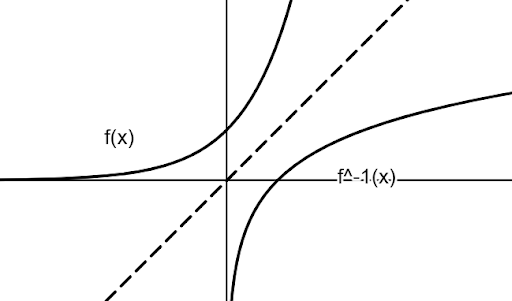
- For example, the inverse of $f (x) = x^{2}$ is $f^{- 1} (x) = x$ , where $x > 0$ .
- Plugging in these values into the composite function yields $(x)^{2} = x$ .

Topic 2.9 - Logarithmic Expressions

Logarithmic expressions are the inverse of exponential functions and are represented as $lo g_{b} (c)$ .
For $lo g_{b} (c) = a$ , $b$ is the base, $a$ is the exponent, and $c$ is the result of $b^{a}$ .
- The logarithm only holds if $b^{a} = c$ , where $a$ and $c$ are constants and $b > 0$ and $b \neq = 1$ .
- If a base is not written, then it is assumed to have $b = 10$ .
  - $lo g (5) = lo g_{10} (5)$ .
A log scale is a type of scale that uses logarithms to show multiplicative change instead of additive change.
- A typical scale is $0, 1, 2, 3$ and so on.
- A log scale using base $10$ will have $1 0^{0}, 1 0^{1}, 1 0^{2}, 1 0^{3}$ and so on. Different bases yield different numbers.
Logarithms may require technology to be solved.
- $lo g_{2} (8) = 3$ since $2^{3} = 8$ .
- $lo g_{3} (14)$ will require technology, since $3^{x} = 14$ cannot be solved through basic arithmetic.
  - The value of $lo g_{3} (14)$ is $2.40217350273$ .

Topic 2.10 - Inverse of Exponential Functions

The inverse of exponential functions are logarithmic functions.
- Logarithmic functions have the general form $f (x) = a lo g_{b} (x)$ with base $b$ , where $b > 0$ and $b \neq = 1$ and $a \neq = 0$ .
We can show that exponential and logarithmic functions are inverses in various ways. All of these under the assumption that $b > 0$ and $b \neq = 1$ .
- From Topic 2.8, $f (f^{- 1} (x)) = f^{- 1} (f (x)) = x$ only holds if $f (x)$ and $f^{- 1} (x)$ are inverse functions.
  - Plugging in $f (x) = b^{x}$ and $f^{- 1} (x) = lo g_{b} (x)$ yields $b^{l o g_{b} (x)} = lo g_{b} (b^{x}) = x$ .
- The graphical property of flipping functions over the line of $y = x$ holds.
  - $lo g_{b} (x)$ can be flipped over $y = x$ to yield $b^{x}$ .
- If $(s, t)$ exists on $b^{x}$ , then $(t, s)$ exists on $lo g_{b} (x)$ .
  - For example, $(3, 8)$ exists on $2^{x}$ . To show that $(8, 3)$ exists on $lo g_{b} (x)$ , plug in and solve for $b$ .
  - $lo g_{b} (8) = 3$ , $b = 2$ . As such, this property holds.
For exponential and logarithmic functions:
- When we increase the input of an exponential function by equal-length intervals, the output is multiplied by the base, meaning that the function changes proportionately.
- When we increase the input of a logarithmic function proportionally, the output changes by equal-length intervals.
  - For example, set $f (x) = 3^{x}$ and set $g (x) = lo g_{3} (x)$ . The table below demonstrates this property.

$x 123 f (x) = 3^{x} 3927 x 3927 g (x) = lo g_{3} (x) 123$

Topic 2.11 - Logarithmic Functions

Logarithms are always either increasing or decreasing, and are either concave up or concave down, meaning that they have no local extrema or inflection point.
Take the logarithmic functions $f (x) = a lo g_{b} (x)$ where $a > 0$ and $b > 0$ with $b \neq = 1$ .
- The function has a vertical asymptote at $x = 0$ that goes towards positive or negative infinity.
- As $x$ increases or decreases without bound, the function also goes towards positive or negative infinity. If one side goes towards one infinity, then the other side goes towards the other infinity.
  - For example, if $x \to \infty lim a lo g_{b} (x) = - \infty$ , then $x \to 0^{+} lim a lo g_{b} (x) = + \infty$
Logarithmic functions have a property where outputs of equal-length intervals allow for proportional changes in the input.
- An output of $4$ in $f (x) = lo g_{3} (x)$ comes from plugging in $x = 81$
- An output of $3$ comes from plugging in $x = 27$
- An output of $2$ comes from plugging in $x = 9$ .
- As the outputs change by equal lengths of one, the inputs change proportionally by a factor of $3$ .
Horizontal transformations can ruin this proportional relationship.
- If $g (x) = f (x + 3) = lo g_{3} (x + 3)$ , the following table illustrates the inputs and outputs.
- The outputs change by equal length intervals of one, but the inputs no longer are proportional to each other.

$x 62478 g (x) 234$

Topic 2.12 - Logarithmic Function Manipulation

Product Property:
- $lo g_{b} (x y) = lo g_{b} (x) + lo g_{b} (y)$ .
- If we have a horizontal dilation of $lo g_{b} (k x)$ , that would be the same as $lo g_{b} (x) + lo g_{b} (k)$ .
  - This is a vertical shift of $lo g_{b} (k)$ units up.
  - A horizontal dilation is identical in effect to a vertical translation for a logarithmic function.
Power Property:
- $lo g_{b} (x^{n}) = n lo g_{b} (x)$ .
- Raising the input of a logarithmic function by a power of $n$ is identical to vertically dilating the function by a factor of $n$ .
Change of Base Property:
- $lo g_{b} (x) = \frac{lo g _{a} ( x )}{lo g _{a} ( b )}$ where $a > 0$ and $a \neq = 1$ .
- The expressions $lo g_{b} (x)$ and $lo g_{a} (x)$ represent two different logarithmic functions, and they are related by the factor $lo g_{a} (b)$ .
- Therefore, every single logarithmic function is related to each other through the change of base.
For a logarithmic function with the natural base $e (e = 2.71 \dots)$ , $lo g_{e} (x) = ln (x)$ .
- Both $lo g_{e} (x)$ and $ln (x)$ mean the same thing, just different notation.

Topic 2.13 - Exponential and Logarithmic Equations and Inequalities

The previous topics about exponential and logarithmic properties allow us to rewrite expressions and solve equations relating exponentials and logarithms.
- One rewriting to know is that $b^{x} = c^{x \cdot l o g_{c} (b)}$ .
Just like for quadratics, there are many times when extraneous solutions may appear.
- After solving for possible values of $x$ , check if the solution is actually valid.
  - For example, take the equation $lo g_{2} (x + 4) + lo g_{2} (x) = 4$
  - $lo g_{2} (x + 4) + lo g_{2} (x) = 4 \to lo g_{2} (x^{2} + 4 x) = 4 \to x^{2} + 4 x = 16 \to x^{2} + 4 x - 16 = 0 \to x = 2.47214 \dots$ and $x = - 6.47214 \dots$
  - Plugging in both of these, notice that $x = - 6.47214 \dots$ is an extraneous solution since $lo g_{2} (- 6.47214 \dots)$ does not exist.
  - Therefore, the answer is $x = 2.47214 \dots$
To find the inverse of logarithmic and exponential functions, recognize that both of these are inverses of each other.
- To remove a logarithmic, use exponentials. To remove an exponential, use logarithms. But otherwise, the same method of swapping the variables of $x$ and $y$ as described in Topic 2.8 can be used.

Topic 2.14 - Logarithmic Function Context and Data Modeling

Logarithms can be used to illustrate a relationship of proportional growth, or repeated multiplication. Logarithms can be used to predict values for dependent values, and find values of independent variables.
There are three ways to construct logarithmic functions:
- The first method is when the question gives the proportionality of the logarithm and the $x$ -intercept.
  - For example, a question may say that for a logarithmic function, an each increase of $1$ in the output corresponds with the input tripling.
  - If the input triples, the proportionality is three. Therefore, the base of the logarithm is $3$ .
  - The question may state that the input is $0$ at $x = 0$ . This is our real zero, and we can construct a logarithmic function with base $10$ that crosses the point $(0, 0)$ .
- Secondly, receiving two points on the logarithm allows us to create a system of equations to solve for the constants in $a lo g_{b} (x)$ .
- Finally, logarithmic regressions are approximations based on logarithmic functions that can be used to create predictions about a scenario.
  - These regressions are constructed using a data set that is inputted into technology like a graphing calculator or Desmos.
    - More information about Desmos can be found on the Desmos guide [link]

Topic 2.15 - Semi-log Plots

A semi-log plot is a plot that has one of the axes logarithmically scaled, usually being the $y$ -axis.
- By scaling the $y$ -axis to follow a logarithmic scale, this means that one unit up represents proportions rather than constant rate of change.
  - A standard $y$ -axis may look like $10$ , $20$ , $30$ , $40$ while a semi-log plot’s $y$ -axis can be something like $3$ , $9$ , $27$ , $81$ , $243$ .
  - Semi-log plots are useful for turning exponential graphs into looking linear.
We can demonstrate that exponential functions can be modeled by semi-log plots through the equation $y = a \cdot b^{x}$ .
- Let us have $a = 3, b = 2$ .
- Using semi-log plots allows us to take the log of the function because of the scaling of the $y$ -axis.
- In this case, let us pick to scale the $y$ axis by $lo g_{2} (y)$ . Therefore, we have the following table:

$x y lo g_{2} y 16 2.58 212 3.58 324 4.58 448 5.58 596 6.58$

The relationship between $x$ and $y$ is exponential, while the relationship between $x$ and $lo g_{2} (y)$ is linear.
- Having a linear graph allows us to do more alterations relating with linear functions, and treat such as a linear function.
We can further demonstrate that exponential functions can be modeled by semi-log plots through the equation $y = a \cdot b^{x}$ and turning it into a linear function.
- Take the log of this function to be $lo g_{c} (y) = lo g_{c} (a b^{x}) \to lo g_{c} (y) = lo g_{c} (a) + x lo g_{c} (b)$ where $c > 0$ and $c \neq = 1$ .
- Notice that the final equation of $lo g_{c} (y) = (lo g_{c} (b)) \cdot x + lo g_{c} (a)$ is analogous to $y = m x + b$ .
  - The slope is $lo g_{c} (b)$ and the $y$ -intercept is $lo g_{c} (a)$ .
- Therefore, taking the logarithm of an exponential function will yield a linear function.

FiveHive