Introduction

Welcome! In this lesson, we’ll focus on the tangent function and how it connects angles on the unit circle to the slopes of lines. Building on your understanding of sine and cosine, you are going to be introduced to a unique function that can be represented in multiple ways including graphically, numerically, and analytically. You will explore how tangent can be expressed as the ratio of sine to cosine, how its graph includes vertical asymptotes and points of inflection, and how transformations such as shifts, reflections, and dilations affect its shape and behavior. By the end of this lesson, you will have a deeper understanding of the tangent function and how it behaves across different representations and contexts.

Essential Knowledge from the CED

According to the AP Precalculus Course and Exam Description (CED), these are the key ideas you’ll be expected to understand about exponential functions for the exam:

Unit Circle Representation: Given an angle in standard position on the unit circle, the tangent function can be interpreted as the slope of the terminal ray. This slope is the ratio of the $y$ -coordinate to the $x$ -coordinate of the point where the terminal ray intersects the circle.
Relationship to Sine and Cosine: The tangent function can also be expressed as the ratio of the sine function to the cosine function. This definition is valid wherever the cosine of the angle is not zero.
Periodicity: The tangent function has a repeating pattern and a period of $π$ . Its values repeat every half rotation of the unit circle.
Asymptotes: Tangent has vertical asymptotes at input values where cosine equals zero. These asymptotes occur at $x = \frac{π}{2} + k π$ , where $k$ is an integer.
Graph Behavior: Between consecutive asymptotes, the tangent function increases continuously and its graph changes from concave down to concave up at the points of inflection.
Transformations: The tangent function can undergo additive and multiplicative transformations.

Adding a constant outside the function shifts the graph vertically.
Adding a constant inside the function shifts the graph horizontally, known as a phase shift.
Multiplying the function by a constant stretches or compresses the graph vertically, and if the constant is negative, it reflects over the $x$ -axis.
Multiplying the input by a constant stretches or compresses the graph horizontally, and if the constant is negative, it reflects over the $y$ -axis.

The Tangent Function and the Unit Circle

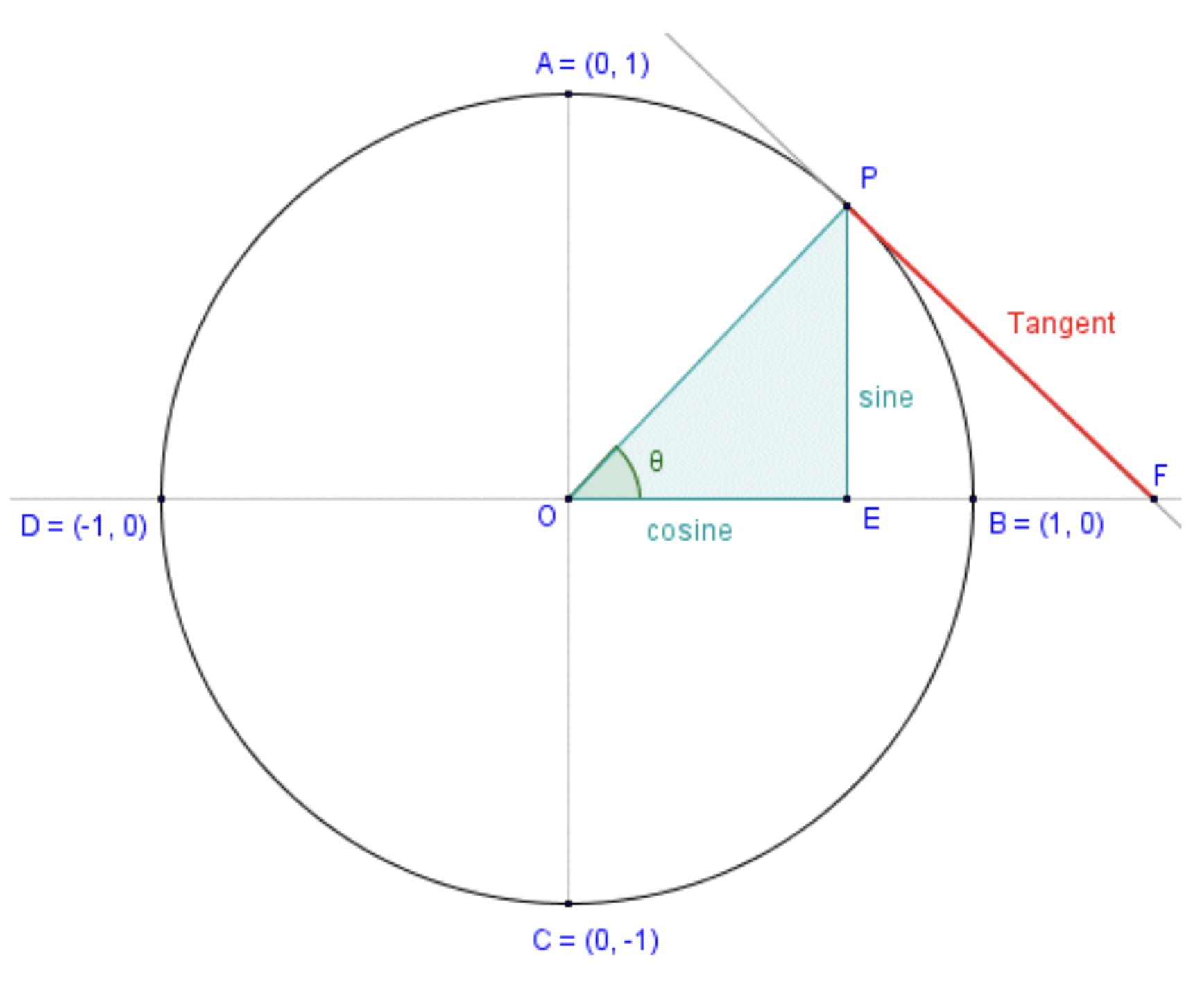
When an angle $θ$ is in standard position, its initial side lies on the positive $x$ -axis and its terminal ray extends from the origin. On the unit circle, which is centered at the origin with a radius of $1$ , the terminal ray intersects the circle at a point $P$ , as shown in the image. This point has coordinates ( $cos θ$ , $sin θ$ ).

As illustrated in the image, the slope of the terminal ray is determined by the change in the $y$ -values divided by the change in the $x$ -values between any two points on the ray. The vertical change corresponds to $sin θ$ , and the horizontal change corresponds to $cos θ$ . Because slope is rise over run, the tangent function gives the slope of the terminal ray. Therefore,

$tan θ = \frac{sin θ}{cos θ}$

where $cos θ \neq = 0$

The red tangent line in the image visually represents this slope, showing how the tangent function measures the steepness of the terminal ray.

Periodicity, Asymptotes, and Behavior of the Tangent Function

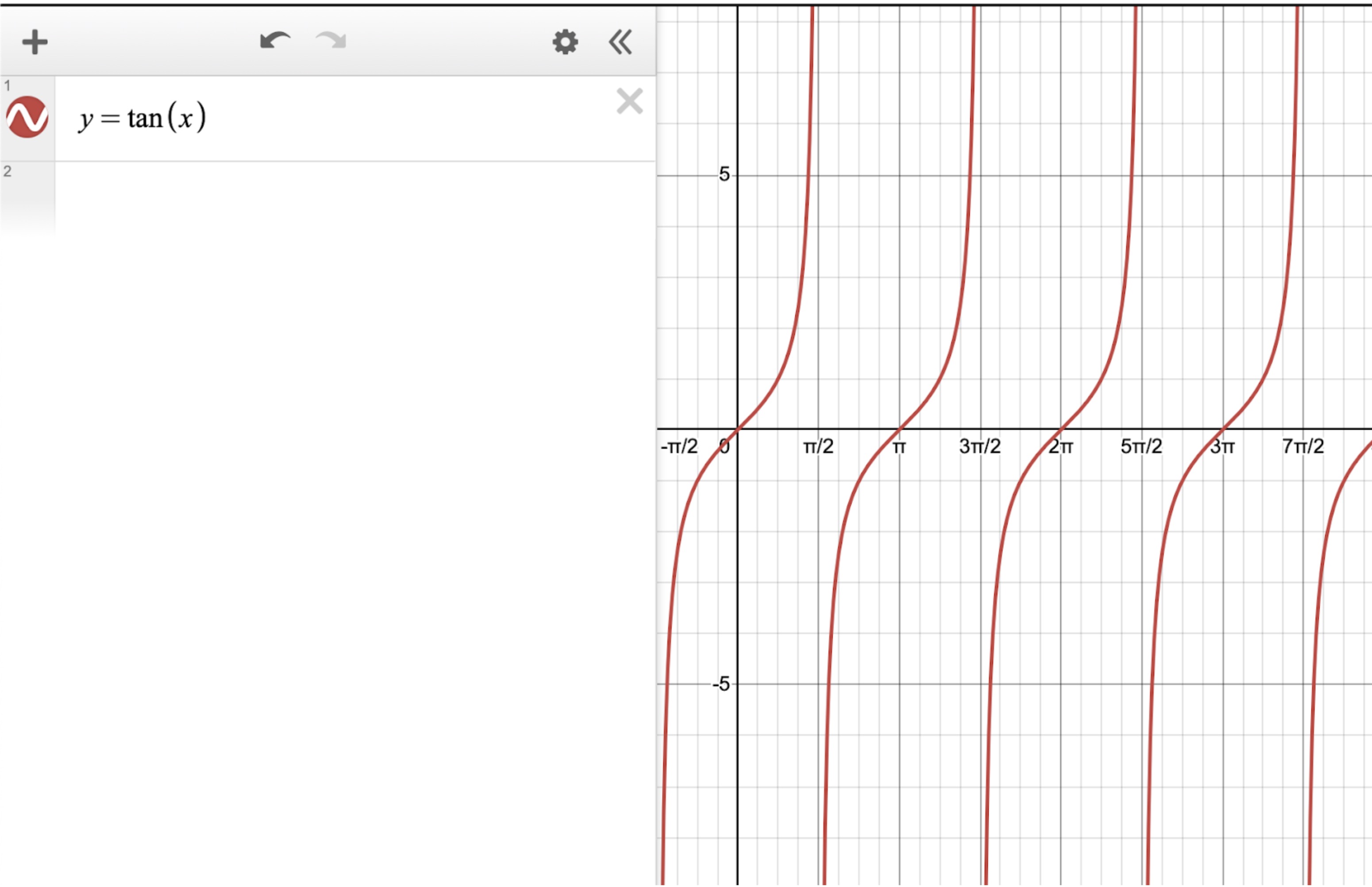
As seen in the graph of $y = tan (x)$ , the period is the length along the $x$ -axis before the graph starts repeating its pattern. For example, at $x = 0$ , $y = 0$ , and as we move along the $x$ -axis, the graph reaches $y = 0$ again at $x = π$ . Between $x = 0$ and $x = π$ , the graph goes through all its typical changes, including approaching positive and negative infinity, which shows a full cycle of the tangent function. Since the graph repeats this same behavior over every interval of $π$ , the period of $y = tan (x)$ is $π$ .

In the graph of $y = tan (x)$ , you can see that at $x = \frac{π}{2}$ there is a vertical asymptote. As the graph approaches $x = \frac{π}{2}$ from the left, $y$ increases toward positive infinity, and from the right, $y$ decreases toward negative infinity. This happens because $tan (x) = \frac{sin ( x )}{cos ( x )}$ , and the function is undefined whenever $cos (x) = 0$ . At $x = \frac{π}{2}$ , $cos (x) = 0$ , so $tan (x)$ cannot have a finite value, which creates the sharp “jump” in the graph.

More generally, tangent has vertical asymptotes at $x = \frac{π}{2} + k π$ , where $k$ is any integer. This formula comes from the fact that cosine equals zero not only at $x = \frac{π}{2}$ , but at regular intervals of $π$ along the $x$ -axis. By adding multiples of $π$ (that is, $k π$ ), we can describe all the points where $cos (x) = 0$ . For example, when $k = 0$ , the asymptote is at $x = \frac{π}{2}$ ; when $k = 1$ , it’s at $x = \frac{3 π}{2}$ ; when $k = - 1$ , it’s at $x = - \frac{π}{2}$ , and so on. These repeating asymptotes occur at equal intervals, which reflects the periodic nature of the tangent function.

Now, if you look at $x = \frac{π}{2}$ , which is one of the asymptotes, you can see that the graph is concave down just after the asymptote. As you move toward the next asymptote at $x = \frac{3 π}{2}$ , the graph increases and changes concavity, passing through $y = 0$ at $x = π$ , where it switches from concave down to concave up. Between these consecutive asymptotes, the tangent function always rises from negative infinity to positive infinity, with the midpoint marking the point of inflection. This pattern repeats between every pair of asymptotes, giving the tangent graph its characteristic S-shaped curve.

Transformations of the Tangent Function

The tangent function, $y = tan (x)$ , can be transformed in various ways. These transformations either shift the graph, stretch or compress it, or reflect it. They can be classified into additive transformations and multiplicative transformations.

Additive Transformations

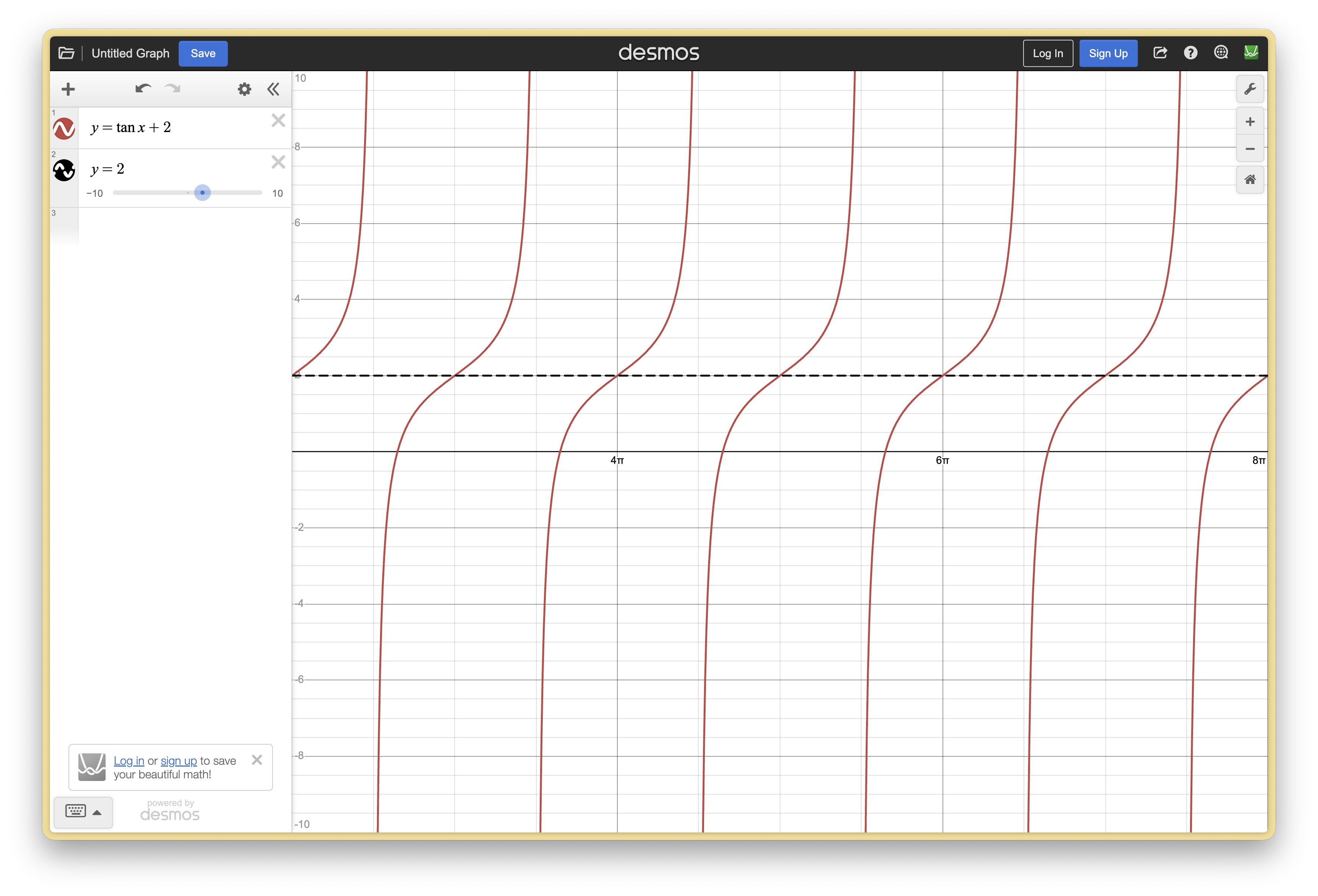
Vertical Translation: The graph of $y = tan (x) + d$ is a vertical translation of the original tangent graph. This means the entire graph, including its points of inflection (where it crosses $y = 0$ ), moves up or down by $d$ units. Positive $d$ shifts the graph upward, while negative $d$ shifts it downward. As you can see in the original graph, at $x = 0$ , $y = 0$ . But when a vertical translation of $+ 2$ units is applied in the second graph, the $y$ -value at $x = 0$ changes to $y = 2$ . This shows that the entire graph, including the points of inflection, has shifted upward by $2$ units, while the overall shape and the positions of the asymptotes remain the same.

Horizontal Translation (Phase Shift): The graph of $y = tan (x + c)$ is a horizontal translation, or phase shift, of the original graph. The graph moves left or right by $- c$ units. For example, if $c = \frac{π}{4}$ , the graph shifts to the left by $\frac{π}{4}$ .

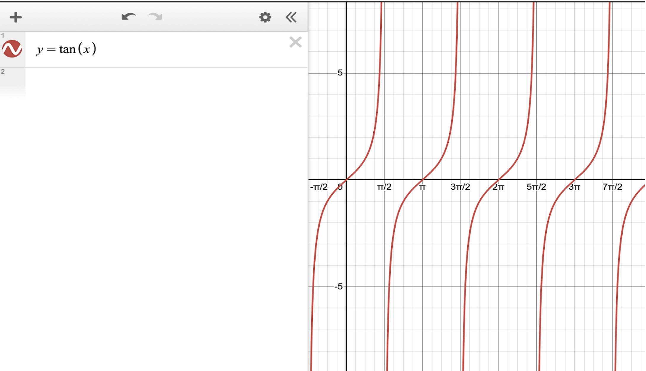
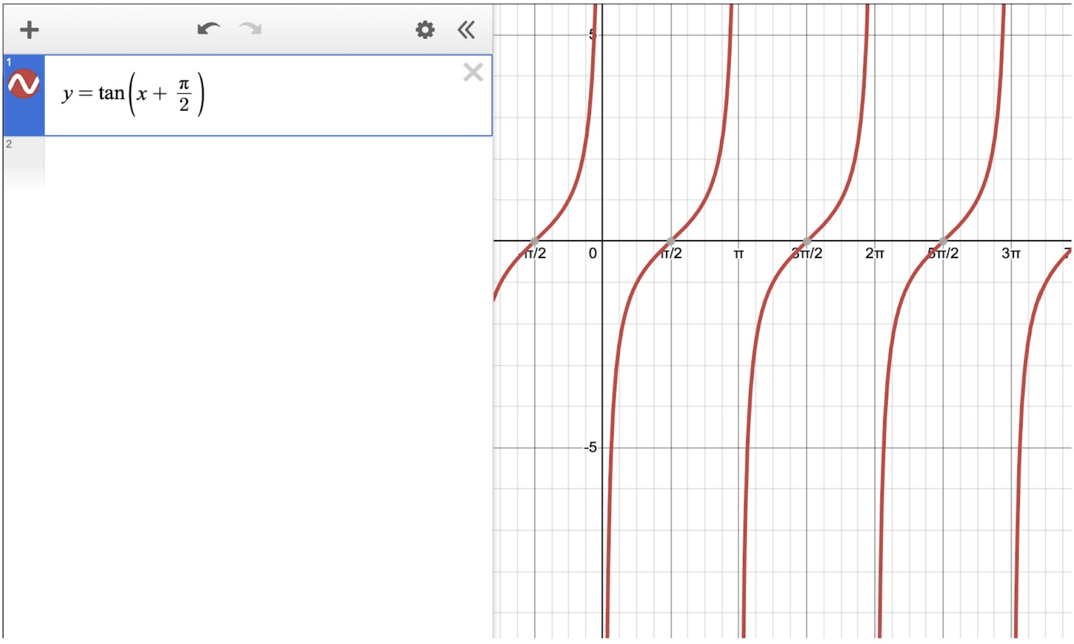
In the original graph, at $x = 0$ , $y = 0$ , and one of the asymptotes is at $x = \frac{π}{2}$ . In the graph of $y = tan (x + \frac{π}{2})$ , the entire graph shifts left by $\frac{π}{2}$ units, so the point that was at $x = 0$ in the original graph now appears at $x = - \frac{π}{2}$ , and the asymptote that was at $x = \frac{π}{2}$ shifts to $x = 0$ . This demonstrates how a horizontal phase shift moves the graph without changing its shape or period.

Multiplicative Transformations

Vertical Dilation (Stretch/Compression): The graph of $y = a tan (x)$ stretches or compresses the graph vertically by a factor of $∣ a ∣$ . If $∣ a ∣ > 1$ , the graph is stretched away from the $x$ -axis; if $0 < ∣ a ∣ < 1$ , it is compressed toward the $x$ -axis. If $a < 0$ , the graph is also reflected over the $x$ -axis.

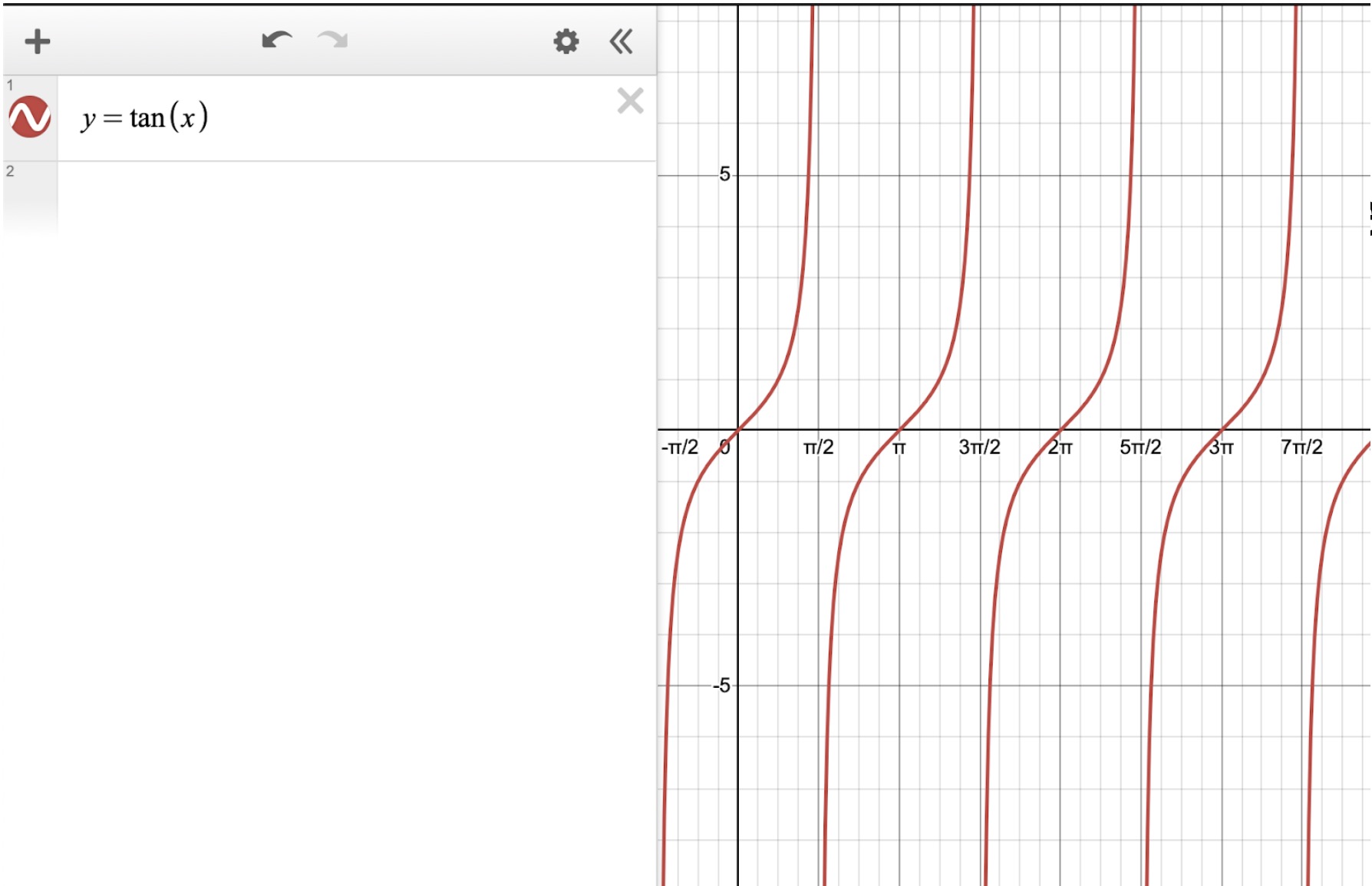
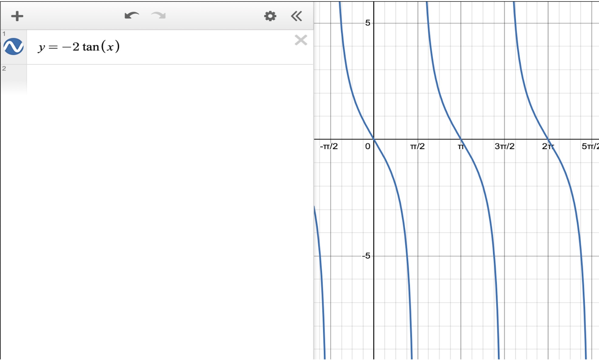
As you can see in the original graph of $y = tan (x)$ , the graph passes through $y = 0$ at $x = 0$ and increases toward positive infinity at its first asymptote at $x = \frac{π}{2}$ . In the graph of $y = - 2 tan (x)$ , the graph is vertically stretched by a factor of $2$ , which makes it rise and fall more steeply. Additionally, because $a = - 2$ is negative, the graph is reflected over the $x$ -axis. This means that what was increasing toward positive infinity in the original graph now decreases toward negative infinity, and what was decreasing toward negative infinity now increases toward positive infinity. The points of inflection, which were at $y = 0$ in the original graph, remain the same, but the overall shape is taller and flipped.

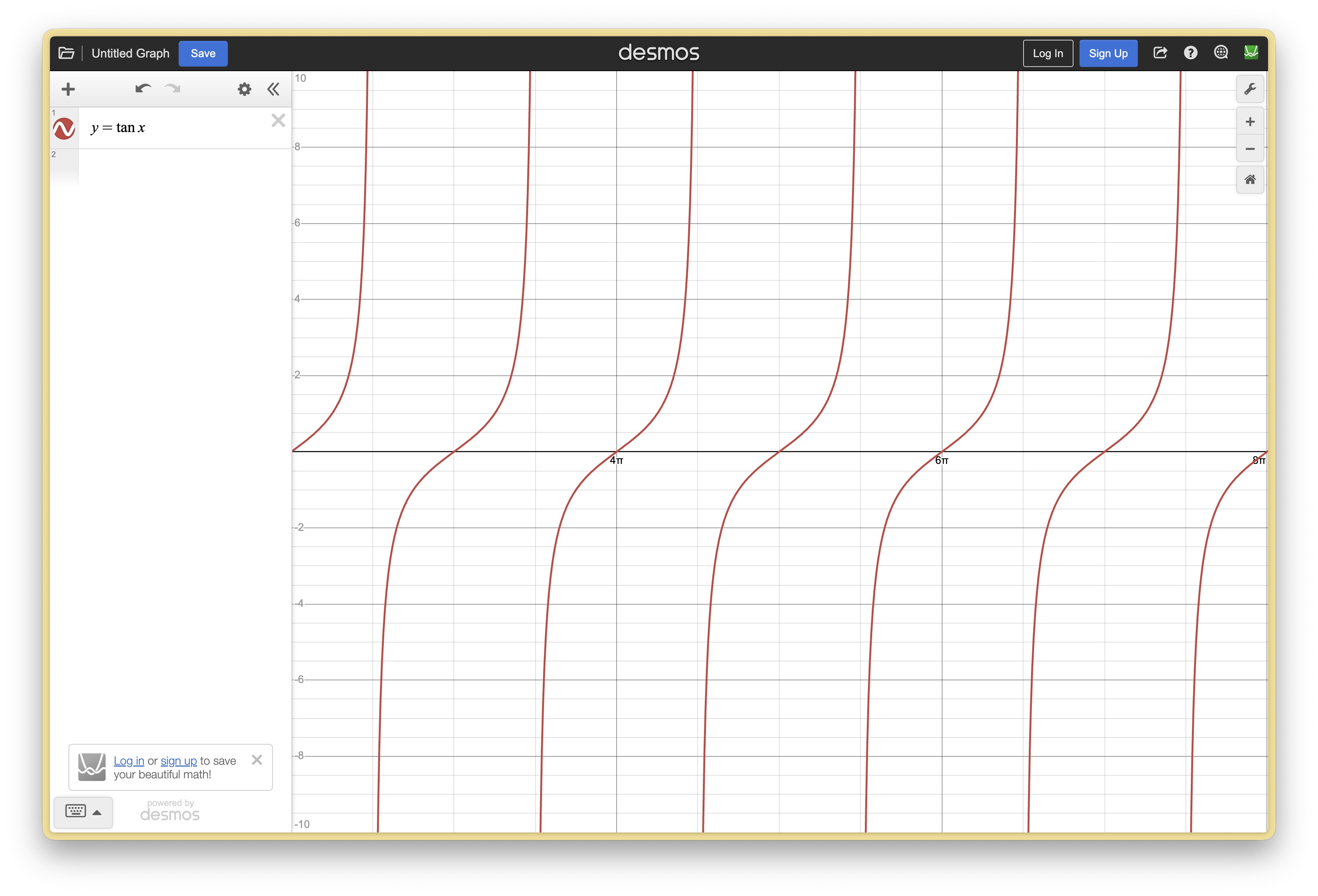
Horizontal Dilation (Change in Period): The graph of $y = tan (b x)$ stretches or compresses horizontally, which changes how wide each cycle of the tangent function is. The period of the graph becomes $\frac{π}{∣ b ∣}$ , so larger values of $∣ b ∣$ compress the graph toward the $y$ -axis, and smaller values of $∣ b ∣$ stretch it away from the $y$ -axis. If $b$ is negative, the graph is also reflected over the $y$ -axis, flipping the left and right sides of each cycle. This transformation changes the spacing of the asymptotes and the width of the repeating pattern, while the overall S-shaped curve of the tangent function stays the same.

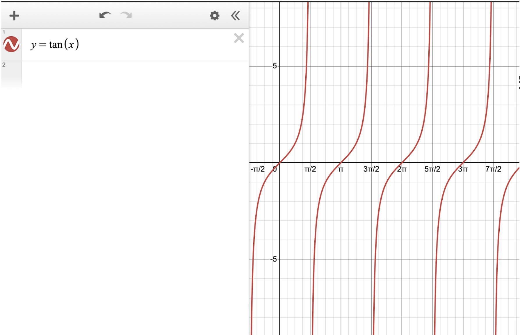
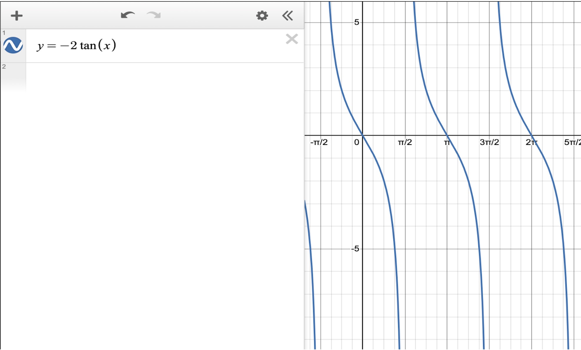
As you can see in the original graph of $y = tan (x)$ , the graph completes a full cycle between consecutive asymptotes at $x = \pm \frac{π}{2}$ . In the second graph of $y = tan (- 0.5 x)$ ,the graph is stretched horizontally because the coefficient $0.5$ is less than $1$ , which increases the period to $2 π$ . Additionally, because of the negative sign, the graph is reflected over the $y$ -axis, so the left and right sides of each cycle are flipped. The asymptotes are now farther apart, and the graph completes one full cycle over a wider interval, while maintaining the characteristic S-shaped tangent curve.

Extension: How Graphing a Tangent Function Works

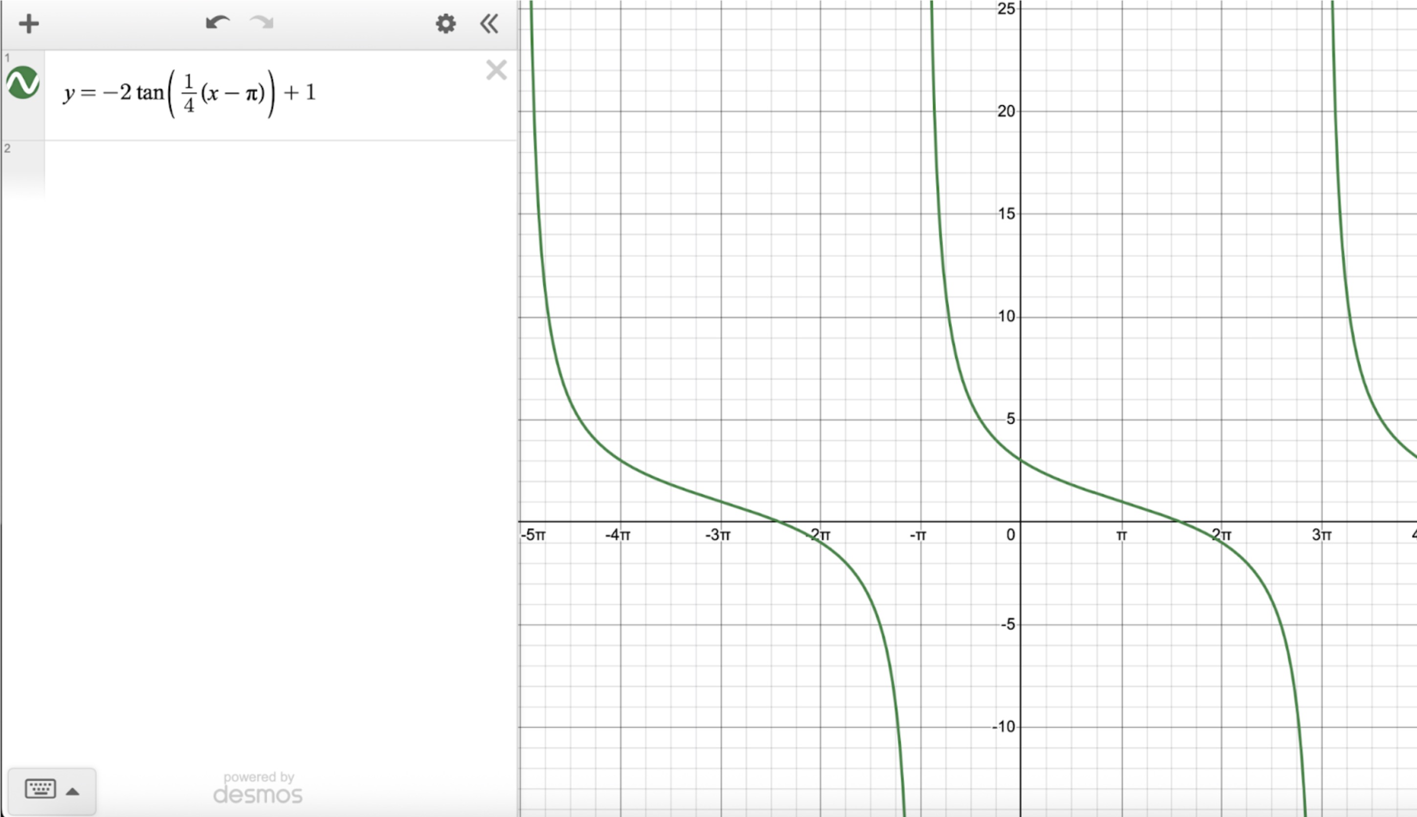
Suppose we have the function $y = - 2 tan (\frac{1}{4} (x - π)) + 1$ . We can graph it step by step:

Step 1: Find the period

For the parent function $y = tan (x)$ , the period is $π$ .For $y = - 2 tan (\frac{1}{4} \cdot (x - π)) + 1$ , the period formula = $\frac{π}{∣ b ∣} = \frac{π}{( 1/4 )} = 4 π$ . So the graph repeats every $4 π$ units along the $x$ -axis.

Step 2: Scale the $x$ -values

The period of the function is $4 π$ . To graph one period, we can divide the period by $4$ → $\frac{4 π}{4} = π$ . This means we can choose $x$ -values separated by $π$ to plot key points.

Step 3: Find the vertical asymptotes

Vertical asymptotes occur where the tangent function is undefined. For the function $y = - 2 tan (\frac{1}{4} (x - π)) + 1$ :

The inside of the tangent is $\frac{1}{4} (x - π)$
Tangent is undefined at $\pm \frac{π}{2}$ , so we set $\frac{1}{4} (x - π) = \pm \frac{π}{2}$ .
Multiply both sides by $4$ → $x - π = \pm 2 π$
Add $π$ → $x = - π$ and $x = 3 π$

So for one period, the vertical asymptotes are at $x = - π$ and $x = 3 π$ . These asymptotes mark the edges of the S-shaped tangent curve for this cycle.

Step 4: Find the new origin

In the original parent function $y = tan (x)$ , the origin is at $x = 0$ , $y = 0$ . This is the point where the graph crosses its horizontal center and the curve changes concavity.

For the transformed function $y = - 2 tan (\frac{1}{4} (x - π)) + 1$ , the phase shift moves this “origin” to the right by $π$ , and the vertical shift moves it up by $1$ .

So the new midpoint of the S-shaped curve is at $x = π$ , $y = 1$ .
This point is also the point of inflection, where the graph changes from concave down to concave up (or vice versa) between the asymptotes.

Step 5: Find the key points between asymptotes

For the parent function $y = tan (x)$ :

To the left of the asymptote $x = \frac{π}{2}$ , there is a key point where $y = 1$ at $x = \frac{π}{4}$
To the right of the asymptote $x = - \frac{π}{2}$ , there is a key point where $y = - 1$ at $@x = -\dfrac{\pi}{4}
These points are halfway between asymptotes, marking the steepest points of the tangent curve

For the transformed function $y = - 2 tan (\frac{1}{4} (x - π)) + 1$ :

The vertical stretch $a = - 2$ multiplies the original $y$ -values by $- 2$
The vertical shift $+ 1$ moves all $y$ -values up by $1$

Since our “origin” starts at $x = π$ :

$π$ to the right → $x = 2 π$ , $y = - 1$
$π$ to the left → $x = 0$ , $y = 3$
Midpoint at $x = π$ , $y = 1$

As you can see in the graph below, all the key points we found are shown for the transformed function. The vertical asymptotes occur at $x = - π$ and $x = 3 π$ . The key points are at $x = 0$ , $y = 3$ and $x = 2 π$ , $y = - 1$ , with the midline at $y = 1$ occurring at $x = π$ . This represents one full period of the function. We can also graph additional periods, as shown in the graph from $x = - 5 π$ to $x = 5 π$ , repeating the same characteristics for each period.

FiveHive