
Introduction
Welcome to topic 3.14!
In this topic, you’ll learn how to construct graphs of polar functions.
Understanding Polar Coordinates and Polar Functions
Last topic, you learned about Polar coordinates, which describe point by an angle and distance .
A polar function is an equation of the form: ,
Where the input (an angle) maps the output (a radius). Thus the graph of consists of input-output pairs (like a rectangular equation). behaves like the “independent variable” (like in the cartesian plane) and behaves like the “dependent variable” (like ).
The most basic form of this is demonstrated in Archimedean Spiral,
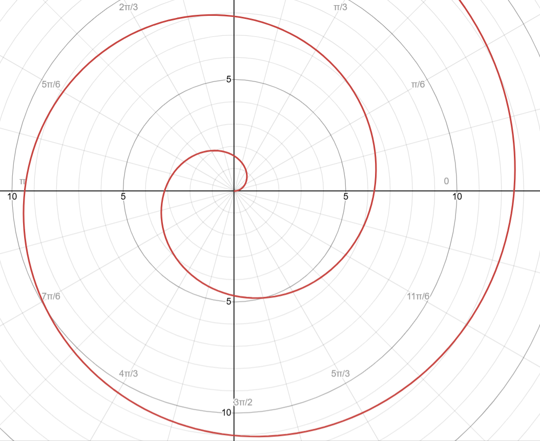
As the angle grows, the radius grows with it.
Other simple forms of Polar Functions include:
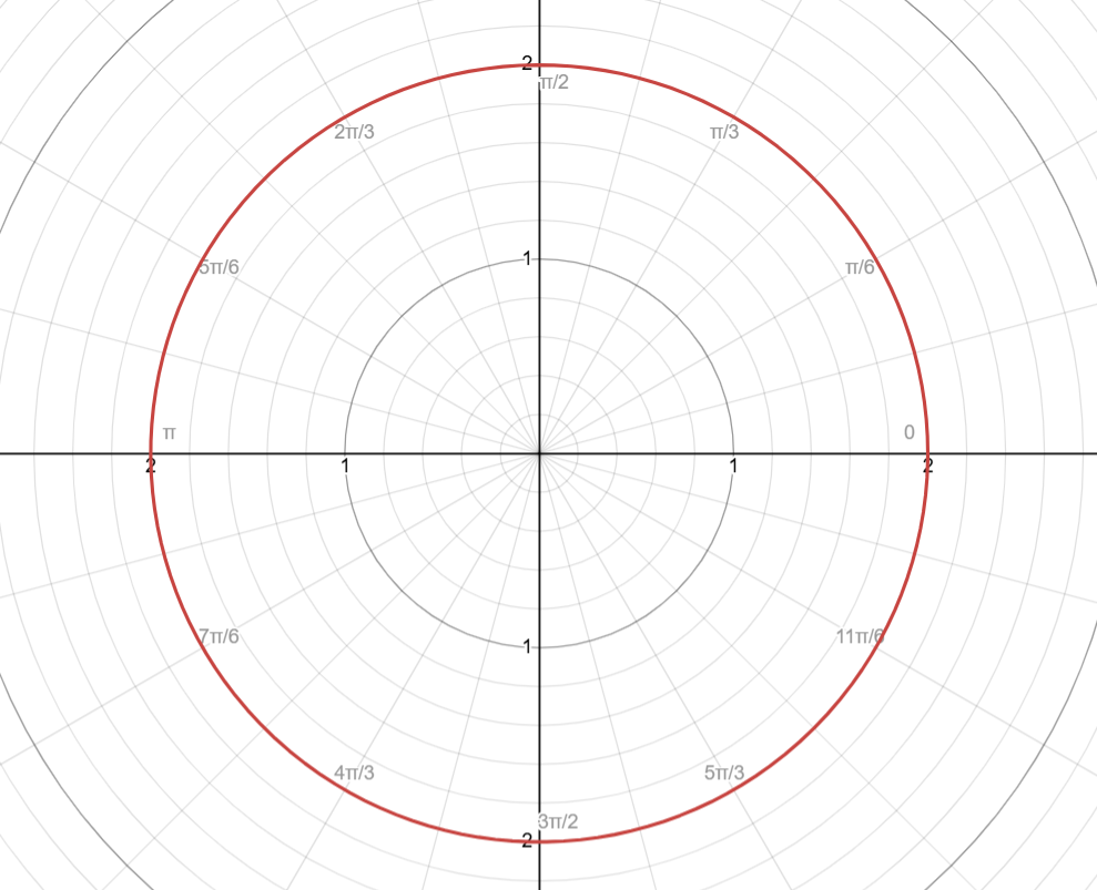
, where is a constant
This means that every point is a fixed distance from the polar. It is simply a circle.
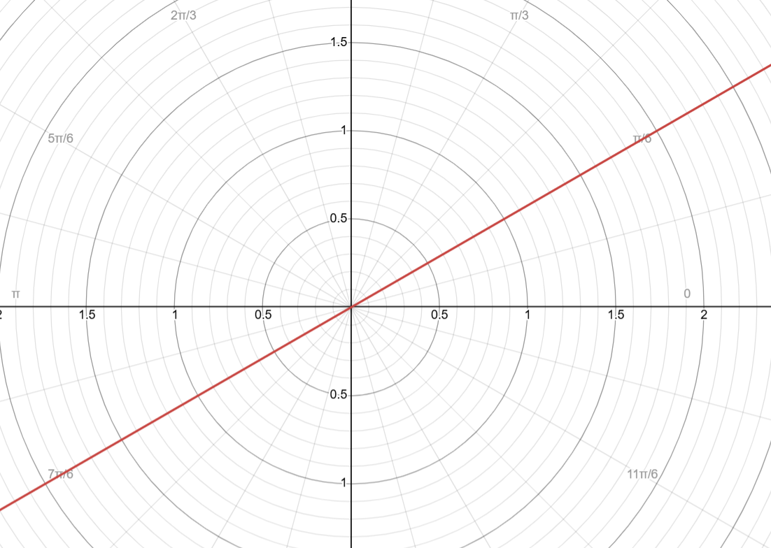
, where is a constant
This means all points lie along a fixed angle. This is shown through a line that crosses through the pole.
How to Graph a Polar Function
Graphing is much like plotting a Cartesian function: we pick values of , compute , plot those points in polar form, and connect them.
The most reliable step-by-step method is simply by creating a table of values:
First, choose a domain (or in this case, your range for ). Usually, we’d choose one full cycle (one full cycle is typically , but as you’ll see later on, some functions repeat on an interval of ).
If the question asks for only a specific interval, then you should pick said interval.
Then, pick sample angles. It is best to pick angles that you should have memorized from the unit circle, like
If involves , pick angles where has simple values like
If involves , pick angles where has simple values like
For , it is often easier to compute from known and values, since has no standard values except
After you pick your sample angles (a.k.a., your domain), you need to compute at each angle.
To do this, simply take your function and beging plugging in your chosen values of .
Now that you have all your coordinates, you can begin plotting them.
I went over how to plot polar points in the last unit, so I won’t go too deep here.
For a quick summary, though, you first draw a ray at angle from the origin, then measure out a distance along that ray.
If , you go out from the pole.
If , you go in the opposite direction.
Finally, connect your points with a smooth curve. This is easier said than done, so hold on before you start answering any problems; we must first go through some of the common types of polar graphs, because without them, you will not be able to correctly connect certain points.
Common Types of Polar Curves
Polar graphs include several “special” curves/graphs with distinctive shapes. The following listed below are some of the most common types of Polar Functions.
Circles (Polar Form)
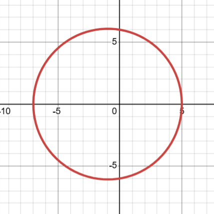
Now, you already know how to graph a circle with center at with a radius . You can convert that into polar and you’d technically have a circle graph.
However, a circle in polar form can also appear as OR , where . These equations both give circles of DIAMETER .
The difference between them is their orientation.
creates a circle centered on the positive -axis.
creates a circle centered on the positive -axis.
Both types pass through the pole when .
They are also both symmetric about the polar axis (note, both the “” and “” axis are called the polar axis. is symmetric about the “-axis” while is symmetric about the “-axis”).
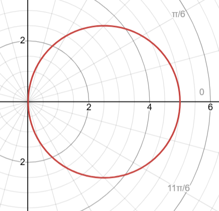
The graph above represents the function . Let’s see why this graph looks like this.
Filling out a table, we see that:
Note, only is needed because for the points repeat (since , the corresponding is negative and sends you back to previous points). Thus, this graph can be modeled by finding points only up to .
Additionally, notice that our value does indeed represent the diameter.
In general, these circles “lie” on the polar axis. As for which polar axis, lies on the “-axis,” while lies on the “-axis.”
If , the graph will be either above or to the right of the pole/origin on the polar axis.
If , it will be below or to the left of the pole/origin on the polar axis.
Rose Curves
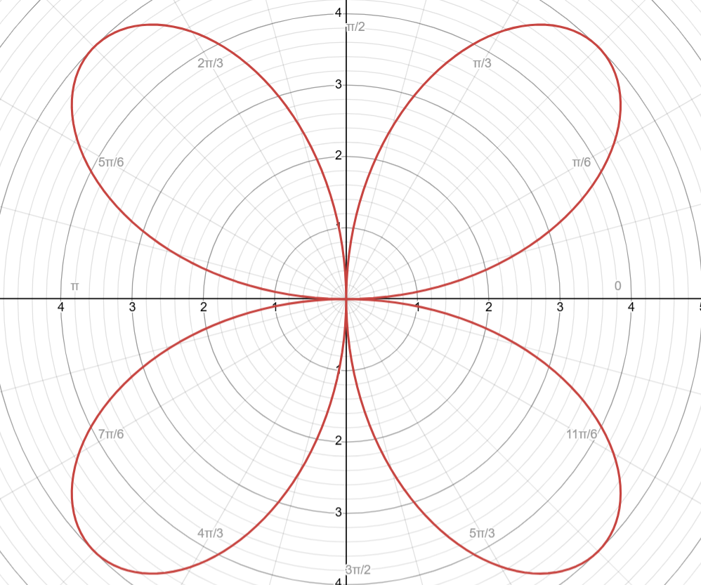
The above is a graph of . It is an example of a rose.
Rose curves have the form: or
Where and is any integer with the condition that , since if it’s equal to , it just becomes a circle.
The graph produces a flower-like shape with “petals.”
The two key parameters are , which controls the petal length, and , which controls the number (and as a result, the spacing) of petals.
There are some general guidelines you can follow to simplify the process:
Number of petals:
If is odd, the rose has petals.
If is even, it has petals.
If you want a cool little experiment, try putting values of that approach or or whatever value; you will see them converge into the specified number of petals.
Orientation (cos vs sin):
A cosine-rose is symmetric about the polar (horizontal) axis, whereas a sine-rose is symmetric about the polar (vertical) axis.
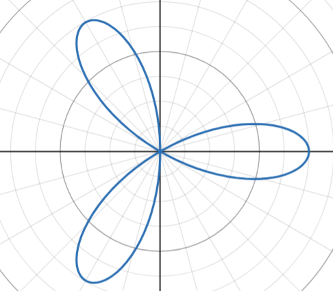
For ,
When is odd, has one petal on the -axis (to the right assuming is positive).
When is even, has a petal on both the -axis and the -axis.
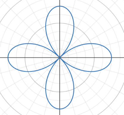
For ,
When is odd, one petal lies on the -axis.
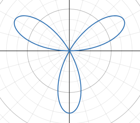
When is even, none of the petals will lie on either axis.
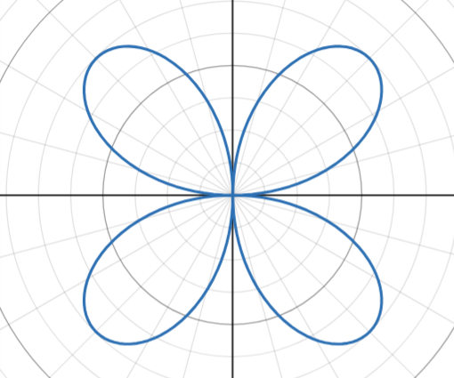
(Note: Transformations can alter these shapes; they will be discussed later)
Petal Endpoints
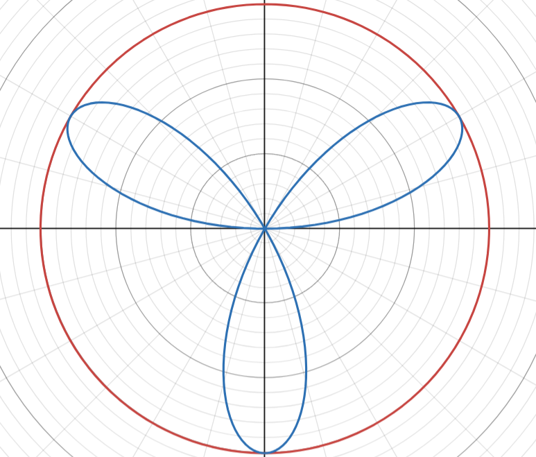
All petals reach out a distance from the pole. In fact, the rose curve is inscribed in the circle : each petal tip lies on that circle.
This makes sense, since the maximum output of any sine or cosine is , so the maximum distance a rose function could go is .
Periodic Behavior:
When is odd, the graph will repeat every . This can also be interpreted as: you only need an interval of , where , to graph the entire function, since after that, the function just begins drawing itself again.
However, when is even, the graph takes an interval of , where , to completely draw the function.
The two main takeaways for this are:
When graphing for when is odd, you only need to find points up to , where is the first point you choose (typically, we choose because it’s the simplest and it is useful for other types of problems).
When finding an interval, you will now be using rather than , if is odd (this will be elaborated later on in the article).
Now, knowing this, you can draw the actual graph. Simply plot the major points (If needed, plotting points that are multiples of can be helpful), then connect them.
Technically, if you’re familiar with the symmetry, you can draw half the petals and just flip them over, though this is not recommended.
However, if you need to find the domain of a specific petal, you must understand how it’s drawn.
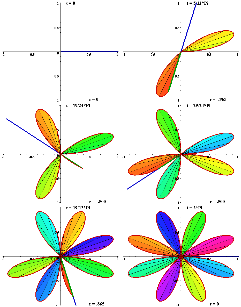
Animations courtesy of National Curve Bank
The rose curve is not like a bouncy ball; it does not repeatedly bounce off of the pole while moving one direction drawing petals. Instead, it follows a certain tangent line, as shown in the graph above.
How the Curve is Traced (as θ increases)
As increases from to (or when is odd), the rose is usually drawn petal by petal (except for one exception which we will talk about).
Each petal is traced when goes from up to and back to over a -interval of length or (depending on whether the graph repeats over an interval of or ).
We typically start a curve when .
Let’s say we have a rose function of cosine:
At , we have .
So the curve begins at the point , which is on the positive -axis.
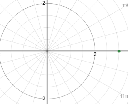
Now, THIS IS THE EXCEPTION (When you are drawing the first petal of a cosine rose function)!
As increases, the function begins to go back towards the pole:
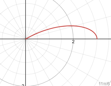
However, instead of completing the current petal, it begins drawing the next:
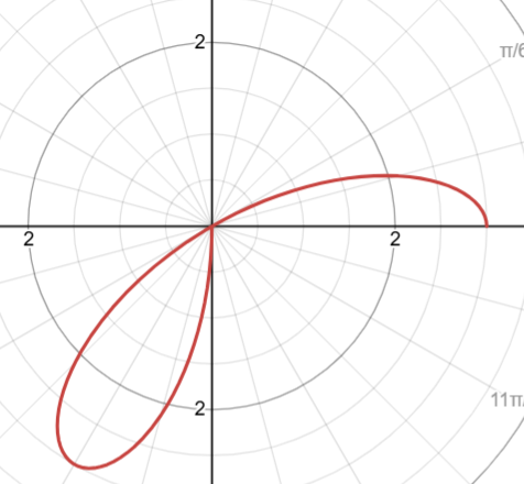
Then, it will complete the next petal
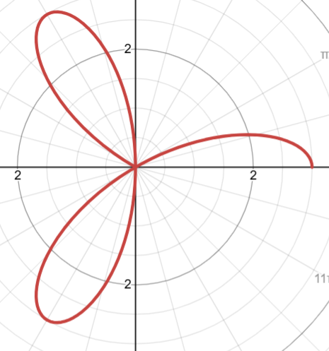
And finally, it will loop around to finish the first petal
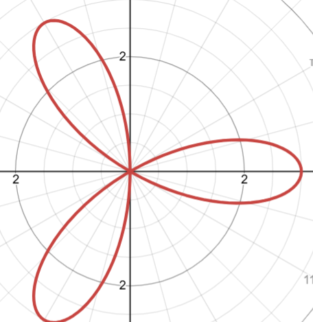
If you’ll notice, the lines/function are always being drawn in a counter-clockwise manner.
If you were to draw this by hand (in the correct order), you will see that your hand is continuously going counter-clockwise.
This will be true for all rose function, meaning you can graph any rose function (in correct order) by
A) finding the major points via a table, and
B) drawing a line through them in a counter-clockwise manner.
However, the main purpose of this is to find a specific interval of the function.
For simplicity, we’ll use a sine function this time.
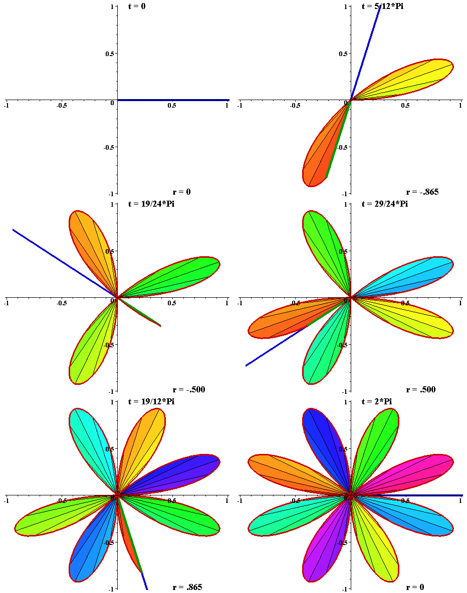
Animations courtesy of National Curve Bank
As you can see, each petal is drawn one after another.
Unlike cosine, sine will always finish a petal before drawing the next.
To start, let’s find the interval of any specific petal.
Because the amount of petals in this function is even, we know that n is even. Specifically, we know that , since there are petals and when is even, the number of petals is .
And for scenarios in which is even, the “period” of the function is .
Each petal is the same in terms of shape; the only difference is what way they face. So, intuitively, it makes sense that each petal is made over equal-length intervals.
Thus, to find the interval of each petal in this graph, we can simply divide by the number of petals:
According to our answer, every time increases by assuming we start from , a new petal will be created.
Is it true? Let's see:
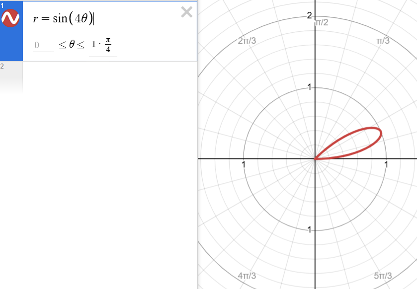
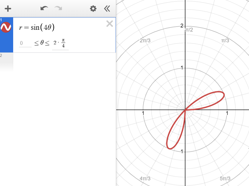
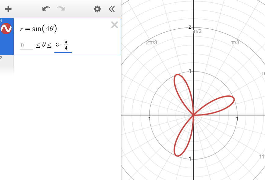
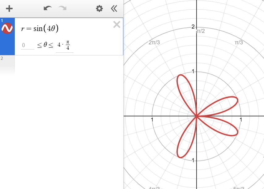
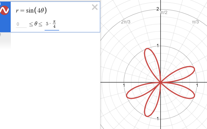
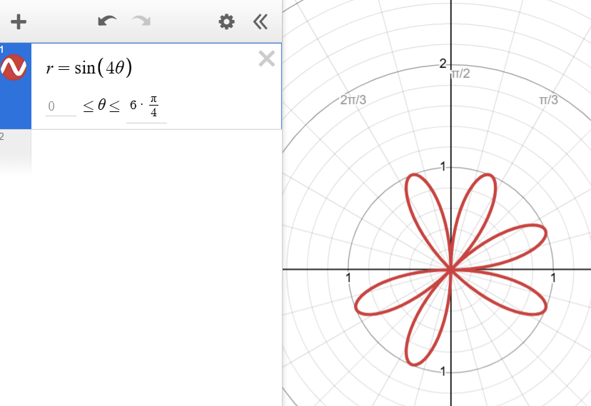
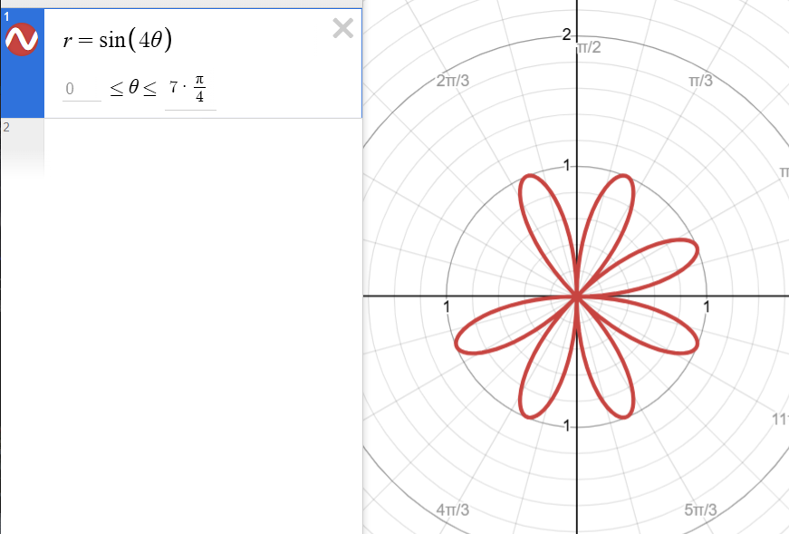
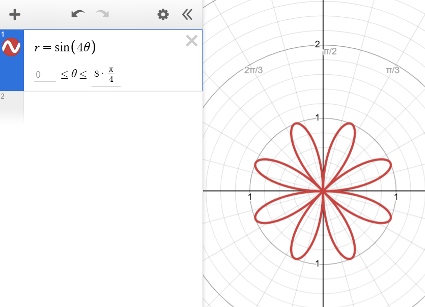
As we can see, every time we add a to our upper bound for the interval of , one new petal is created, confirming that the interval-length for each petal is .
Intuition can also guide you from here; the interval-length of half a petal is half of the petals’ interval-length. In other words, from the pole to the tip of a petal, there is an interval-length (Remember, this is for the function ).
Limaçons
Limaçons (coming from the French word, “snail”) are polar curves in the form
Or
Depending on the constants and , they take on several shapes.
When ,
The Limaçon will be in the shape of a heart, and is thus called a heart shaped Limaçon. It is also called a Cardioid.
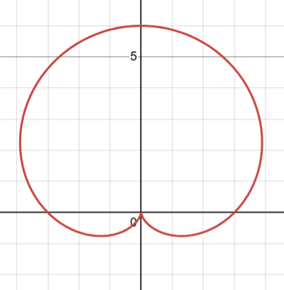
When ,
The curve has an inner loop, and is thus called an inner-loop Limaçon.
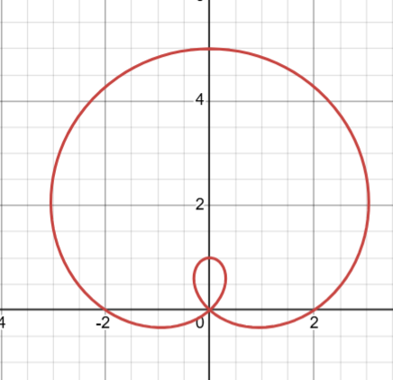
When ,
This Limaçon is called a Dimpled Limacon.
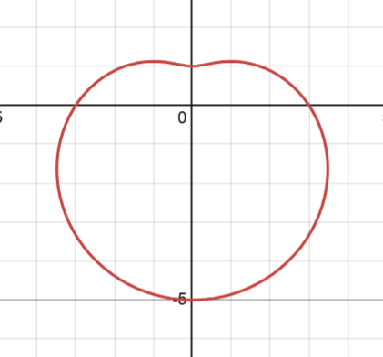
And when ,
(Note: Convex Limaçons are NOT to be confused with circles. As you will learn later, Convex Limaçons are not centered at the pole)
Graphing most Limaçons are not difficult; usually, you can simply find key points and graph from there (although some difficulty may arise with the inner loop, which will be elaborated upon later).
In the next section, you will read about the significance of these keypoints.
Key Points of Limaçons
Generally, for any Limacon, you must find the points at which the function crosses both polar axes.
However, a useful fact for any limaçon is that the maximum radius is |a|+|b| and the minimum (if positive) is .
For (dimpled case), the “dimple” point is at (will be elaborated upon later)
Cardioids/Heart shaped Limaçons
When graphing Cardioids, the points you absolutely need to find are the points at which , , , (note, you do not need because that is when the function begins repeating itself).
To find the points, you simply plug in each value of and you will receive its corresponding . After, you can simply graph it to get a general shape of your function.
As for other points you can graph to make your graph more accurate (which are HEAVILY recommended but are not completely necessary to understand the general shape), you can simply follow the same rule for roses:
If your function uses cosine (if the function looks like it’s shifted right or left), then use angles that are multiples of for values that come out cleanly.
If your function uses sine (if the function looks like it’s shifted up or down), then use angles that are multiples of for the same reason.
Once you have your points, you can simply connect the dots.
If you are asked for a specific interval, you can simply graph the points that have a in that interval (of course, if the interval starts with a value of that is not shared by one of your points, you will need to find the coordinate for the value of asked)
Inner-loop Limaçons
After some practice, knowing how to connect the dots for an Inner-loop Limaçon becomes easy (it’s really the only way you can get better at it, a.k.a., by going through more examples).
However, the hard part is finding specific intervals, which, if you’re given an inner-loop Limaçon, is most likely what’s being asked.
First, find where (the pole intersections).
There should be solutions. If there are not, you most likely do not have an inner-loop Limaçon.
Use these solutions as boundaries. If asked for a theta-specific interval, it typically (note, not always) starts at one of these solutions and ends at the other. Occasionally, however, it may start at one of the intersections with the polar axis.
Typically, when asked for an interval, it will have bounds that lie at the farthest point from the pole (a multiple of or depending on whether your function is sine or cosine), one of two (or both angles) that lead to (aka the two intersections at the pole, or the farther point on the inner-loop from the pole.
There will be practice problems provided at the bottom of this article.
Convex Limaçons
Convex Limaçons are NOT the same circle polar functions you learned earlier.
The difference lies in the fact that they are not centered at , or the pole.
Other than being able to tell the difference, there is not much to them. You simply plot your points and connect them in a circular fashion.
Note: Convex Limaçons do not share the behavior of circles, that being, they take to complete a revolution instead of . This is true for all Limaçons.
Dimpled Limaçons
Dimpled Limaçons are actually a bit hard to graph, especially since you can’t exactly see the dimple sometimes.
First, determine whether the function uses cosine or sine.
If it is cosine, the dimple will be on either the left or right.
If it’s sine, then it will be on the top or bottom.
Second, you must find the minimum and maximum distance from the pole. The maximum and minimum r-values are crucial for seeing the dimple’s extent.
Now, you do not need to find every major point on the graph to find the min and max distance.
Instead, you just need to know that,
is the maximum distance from the pole
And
is the closest positive distance to the pole.
This point is the dimple.
After plotting the other major points previously mentioned that apply for any polar function, simply connect the points smoothly and you’ll be done.
For finding a specific interval, it’s essentially the same as a circle, except that now instead of the function repeating every , it repeats every .
Finding Polar Equations Given a Graph
To find the specific equation or that is represented by a given graph, you must identity the type of symmetry (which trigonometric function is being used) and measure the radial extrema along the axis of symmetry.
First, we must establish the type of function. Symmetry about the horizontal polar axis implies the use of , while symmetry about the vertical polar axis implies the use of .
Next, the maximum and minimum radial distances along this axis must be measured.
For any Limaçon (not just the dimpled variety), the maximum distance from the pole to the farthest edge of the curve is .
However, for the closest point to the curve, the method varies depending on the type.
For Convex, Dimpled, or Cardoids, the positive distance between the closest point to the pole and the pole is given by .
However, for Inner-Loop shapes, represents the distance to the tip of the inner loop, but the algebraic value is negative to form the loop.
We define as the signed radius . If the inner loop extends units, then .
As for why this is true, simply creating a table of points and graphing their respective radius will show you why.
Once you have these two measurements, you can solve for a and b using this simple system:
Lemniscates
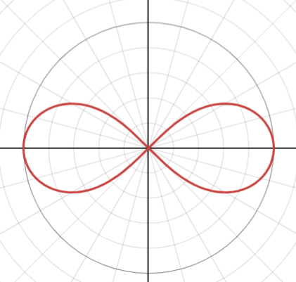
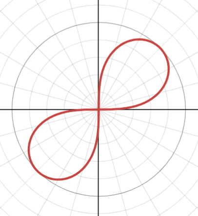
Lemniscates (Latin for “ribbon”) are figure-eight-shaped curves centered at the pole. They are fundamentally different from Limaçons and Roses because their equations involve , which imposes special restrictions on where the curve can exist.
Note: Lemniscates rarely appear on the AP exam! So far, a lemniscate has not appeared on an AP exam, however, there may be one multiple-choice question on a future exam featuring a lemniscate.
The two standard forms for lemniscates are the following:
They look like this:
In both equations,
represents the maximum distance from the pole to the tip of either loops.
Once again, orientation will be based on the trigonometric function (sine or cosine).
If the function uses cosine, then the loops are aligned along the axis (the horizontal polar axis) or the axis (the vertical polar axis)
If the function uses sine, the loops are aligned diagonally along the lines or .
Graphing Lemniscates
The Domain Restriction
Since the equation for a lemniscate contains the term , the right side of the equation (with the trig functions) must be positive for to be a real number. If it were negative, would be undefined. This requirement creates angular “gaps” in which the curve does not exist. To demonstrate this concept, let’s try graphing the function .
(Note: is the same as graphically. Since is also the same graphically as the two polar functions above, there is no need to graph the square root variants of this lemniscate curve.)
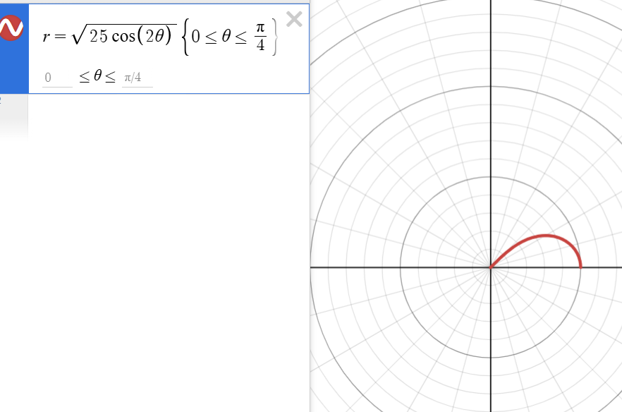
The first interval is . Intuitively, the next portion of the graph should be drawn when reaches . However,
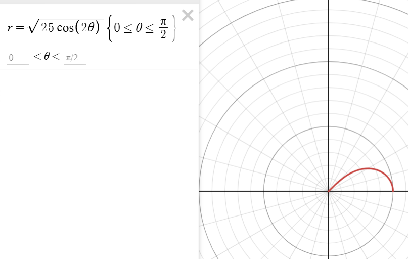
nothing changes. Let's see what is going on in the background.
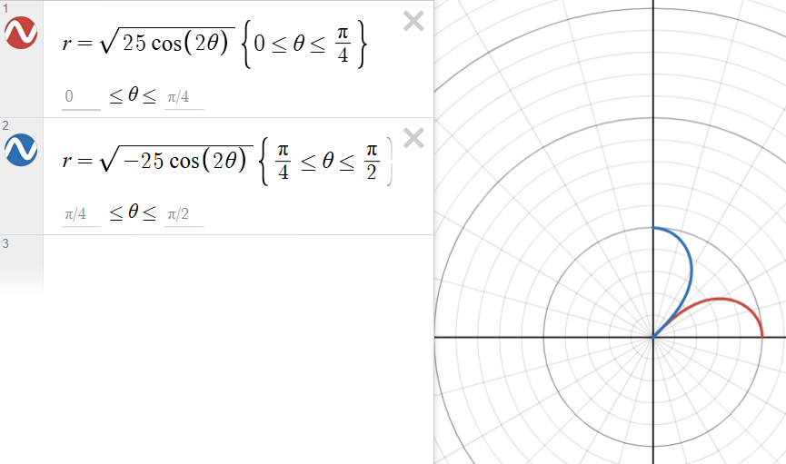
As we can see, when goes from to , the graph of is drawn. Then, when theta goes from to , the function of is drawn. This is because from to , is negative, so if we add a negative sign inside the square root, we can see what’s happening between the “gaps.”
Let’s see what happens as we continue.
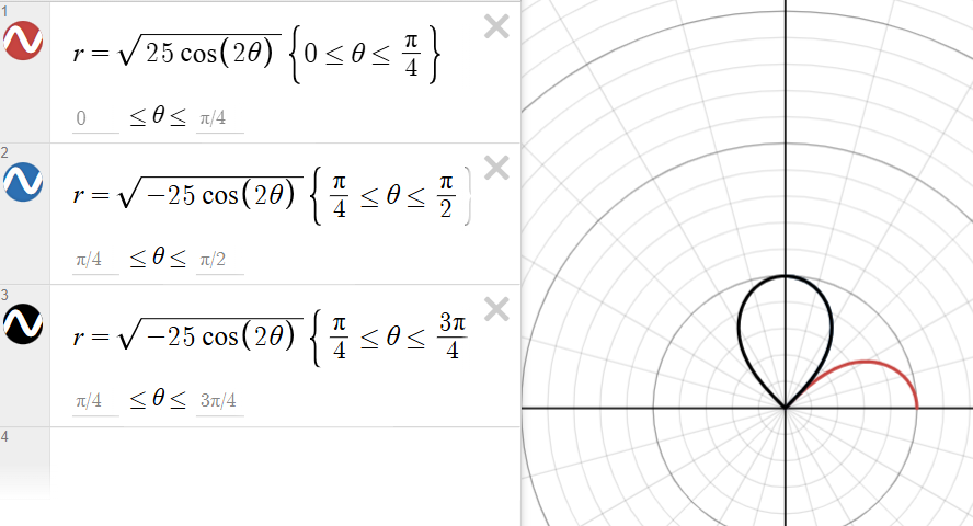
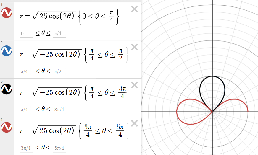
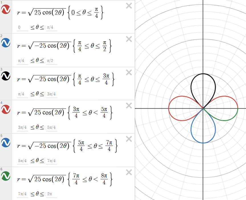
Thus, to trace one loop of a lemniscate, you must find the angles () where the curve begins and ends at the pole .
For , the curve is only traced where . One full loop is traced from to .
For , the curve is traced only where . One full loop is traced from to .
Plotting the Two Loops
Fortunately, actually plotting the lemniscate is nowhere near as hard as graphing something like the inner-loop. When you solve the equation for , you get . For every valid angle , there are two corresponding radii: a positive and a negative Plotting both of these points is what automatically generates the two loops of the lemniscate shape.
Technically, if you’re careful, you can find one side of the lemniscate and simply “copy it over” whatever polar axis it’s symmetric to; this distance between the farthest point from the pole will be the same, only its direction will be reversed. As for connecting the points, there’s not much to it. Unlike the rose polar function or the dimpled limaçon polar function, lemniscates don’t have any special areas where they differ from the natural curve. If need be, you can find points in between the angles theta that correspond to the max distance from the pole, assuming the value theta is a valid angle.
Finding the Lemniscate Equation Given a Graph
To derive the equation from a graph, you only need to perform two steps:
First, identify the function type. Once again, if the loops lie flat on the axis or the axis, use the cosine function for lemniscates (Note: When it is on the axis, it means the inside of the square root has an added negative sign:
If the loops lie diagonally, use . If the loops are in quadrants 1 and 3, then the normal equation works. However, if they are in quadrants 2 and 4, then the function has a negative added in the square root: .
Then, measure the length . Measure the distance from the pole to the tip of any loop. This value is . Remember to square this distance to find for the final equation.
Practice Problems
- What is the center and radius of the circle given by ?
- Write the polar equation of the circle with center and radius
For Questions 3-12, graph the functions given. It is suggested that you construct a table of values first before graphing each function.
For Questions 18-20, name and graph the following polar functions:
For Questions 21-23, convert the following polar functions into rectangular form:
For Questions 25-26, convert the following rectangular functions into polar form. Use trigonometric identities to simplify the final answer.
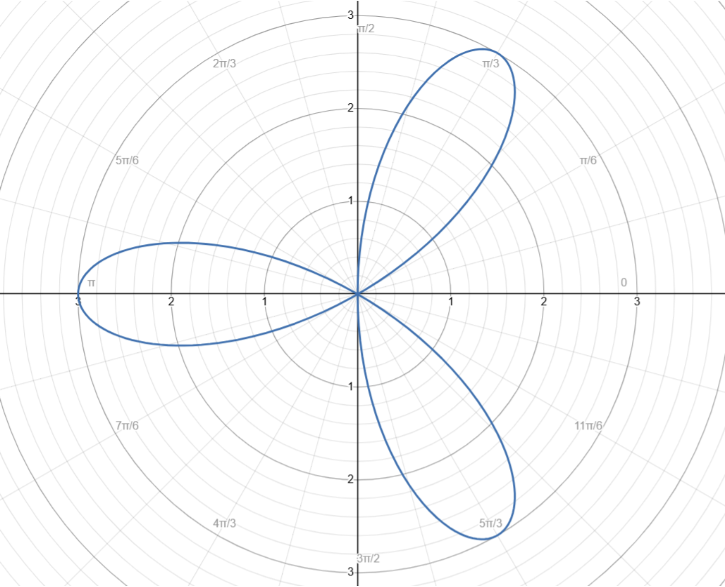
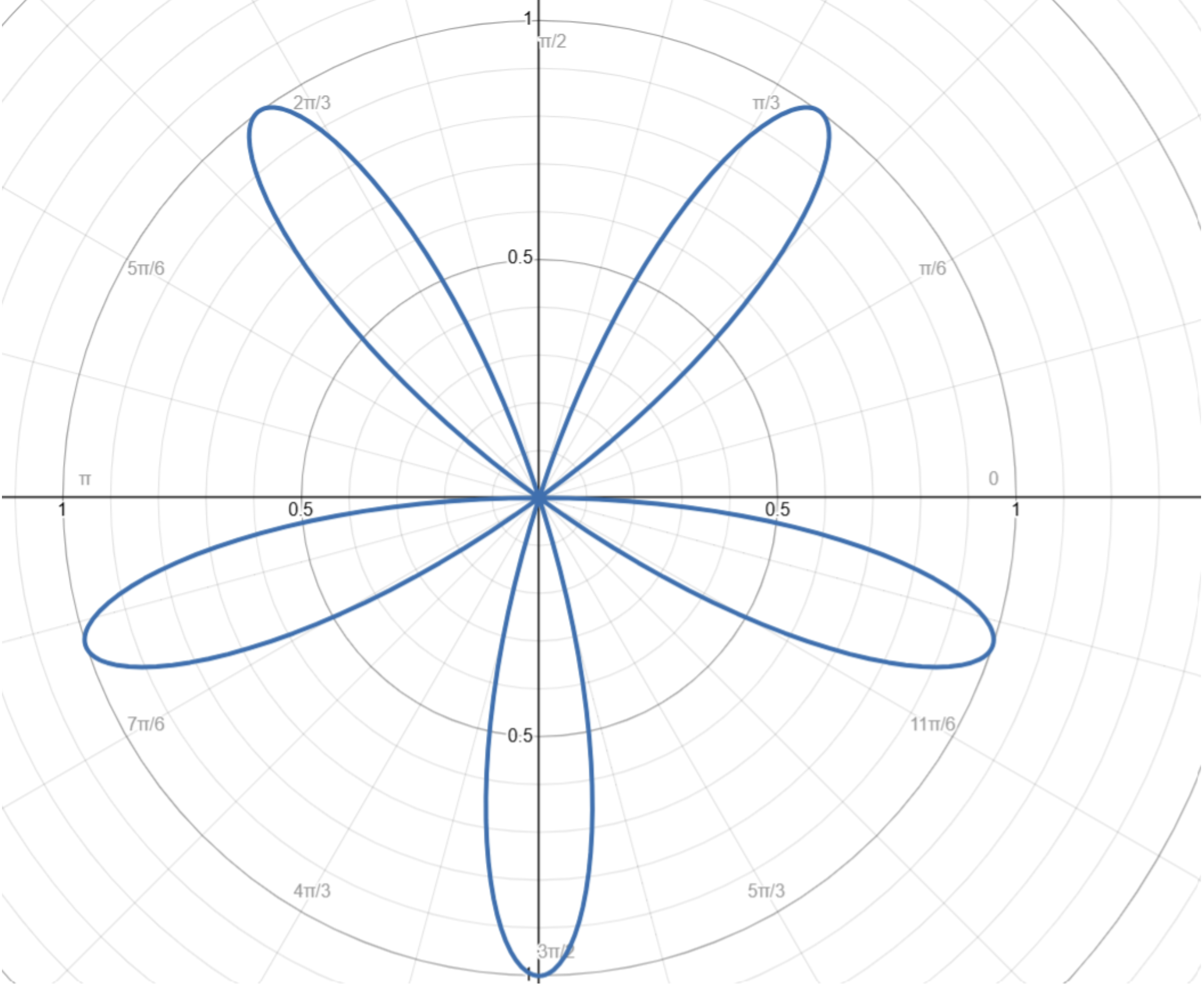
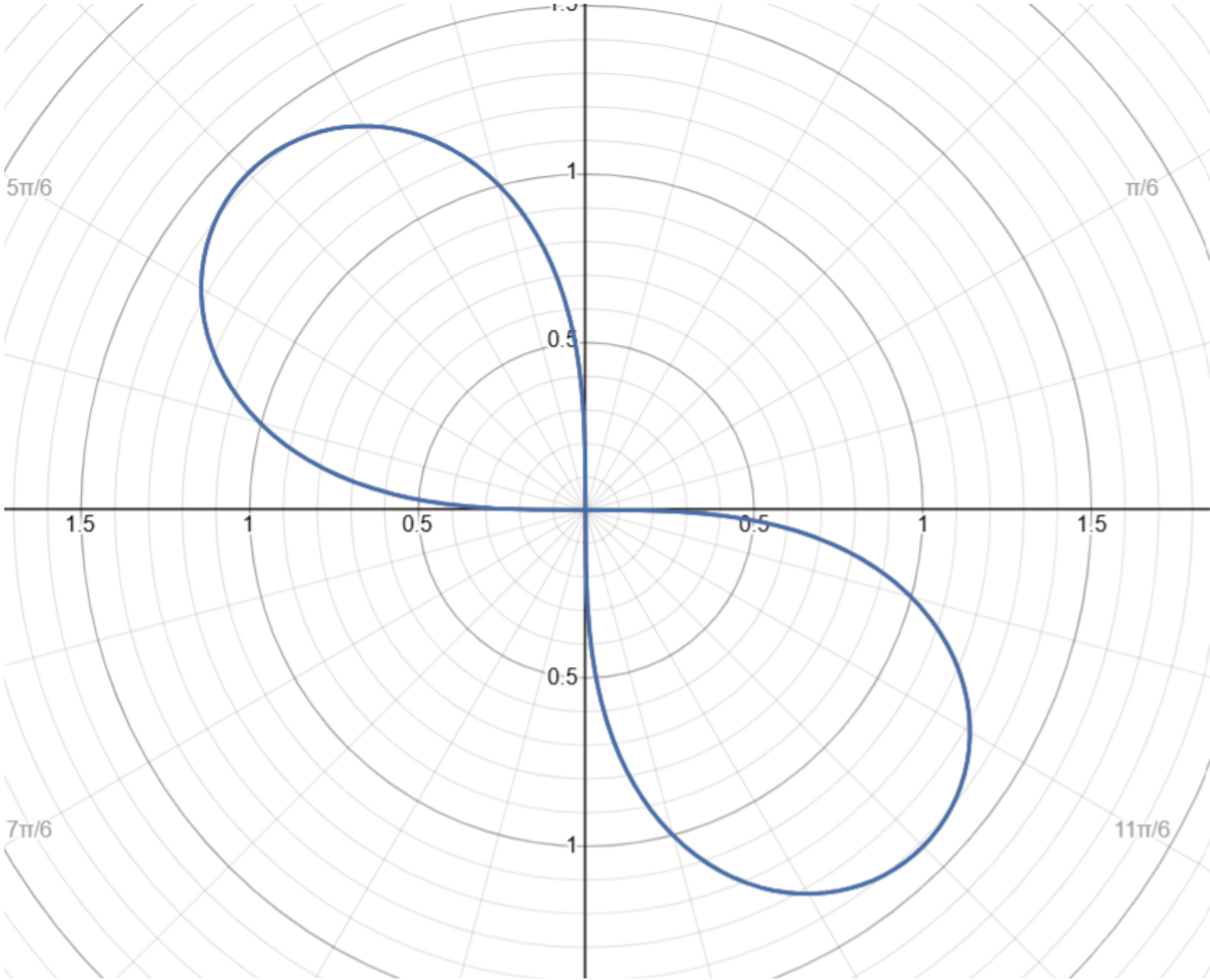
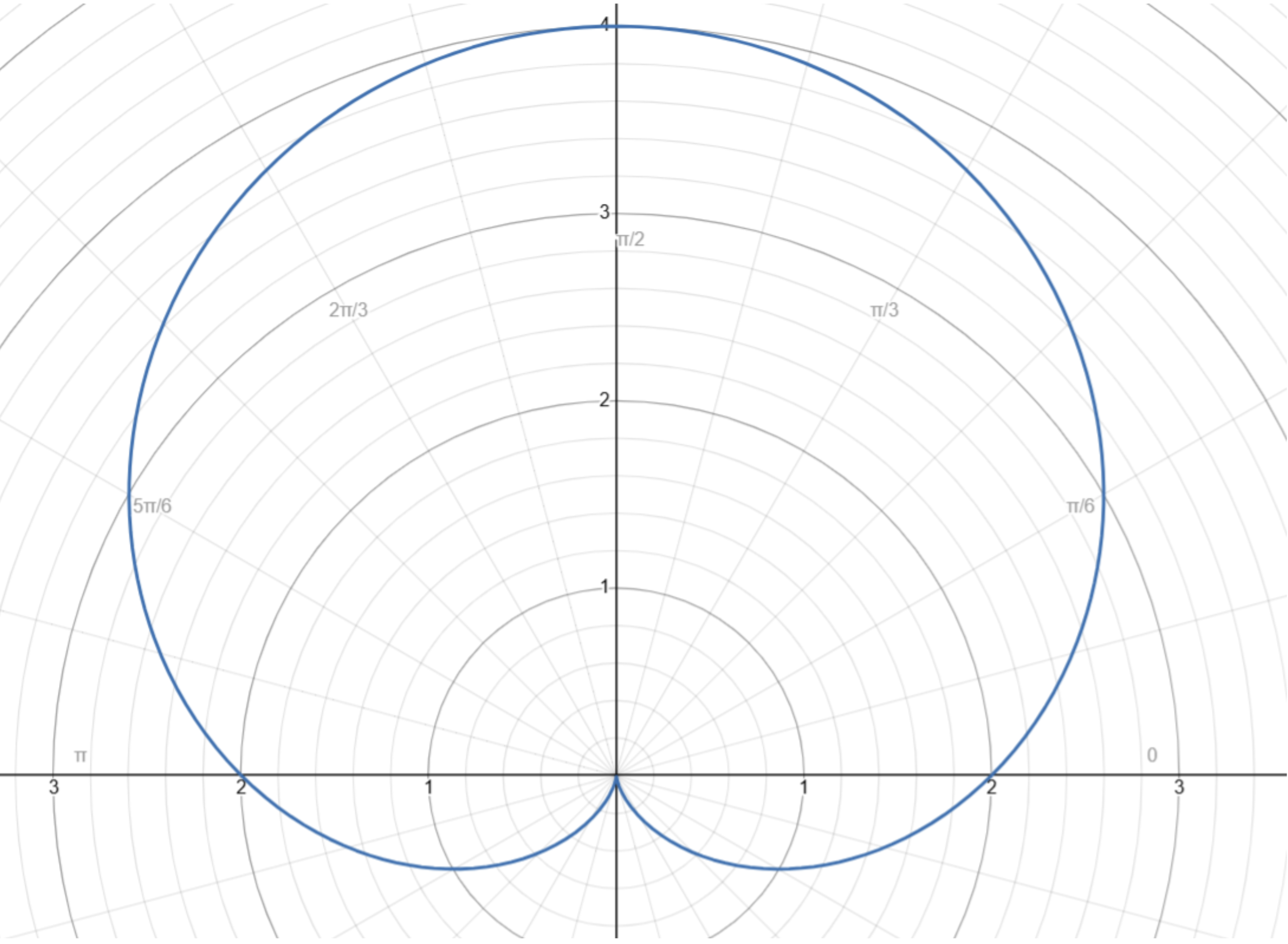
For Questions 27-28, write the equation that corresponds to the graph shown. Additionally, name the type of graph shown.
Question 27
Question 28
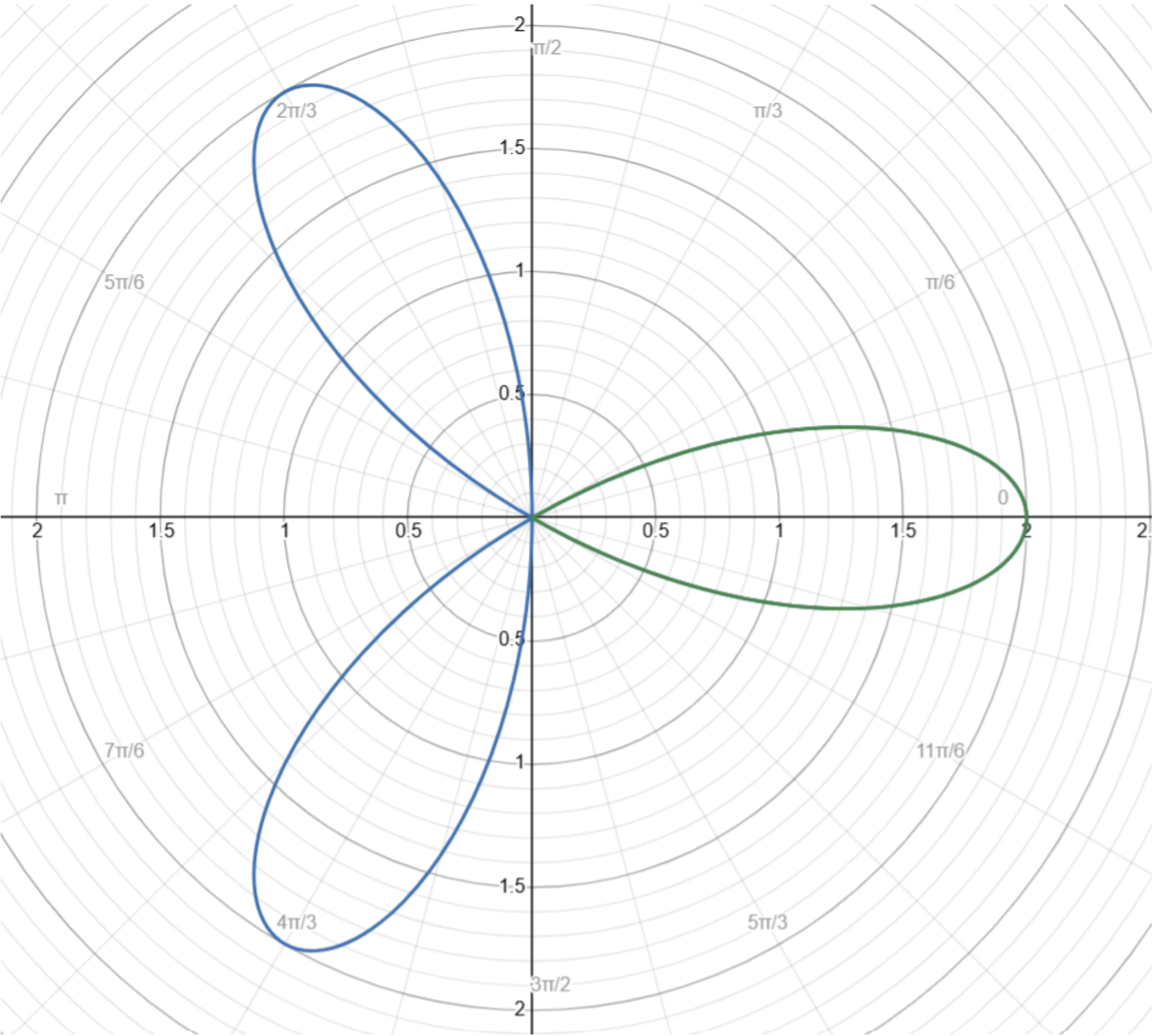
For Questions 29-31, provide the interval for the dashed portion of the graph. The domain of the function is .
Question 29
Question 30
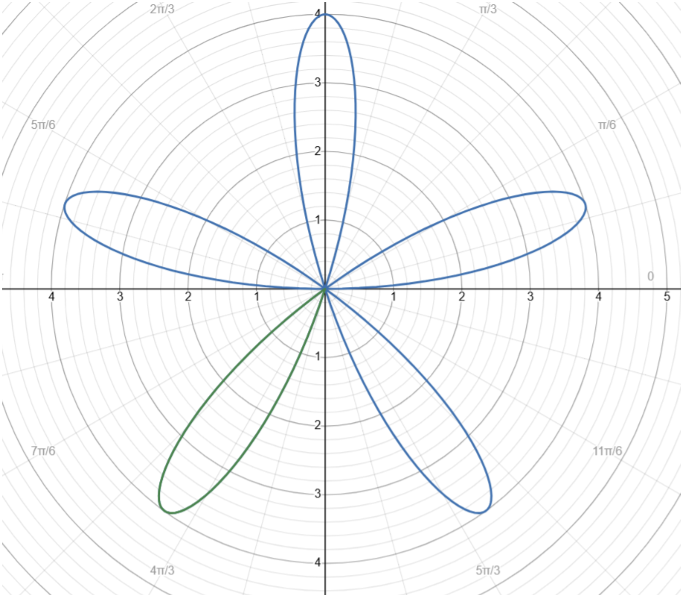
Question 31
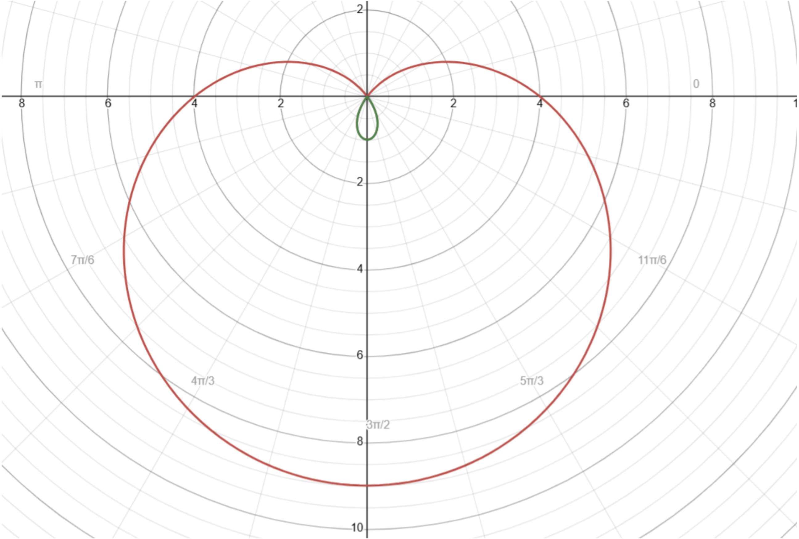
Solutions to Practice Problems
-
-
Multiply both sides by r:
-
Add 16 on both sides to complete the square:
-
Factor:
- This is simply a circle. The center of the circle is and its radius is
-
Multiply both sides by r:
-
First, let’s write the rectangular formula:
-
Substituting and :
-
Using the Pythagorean identity, :
- The answers are are and
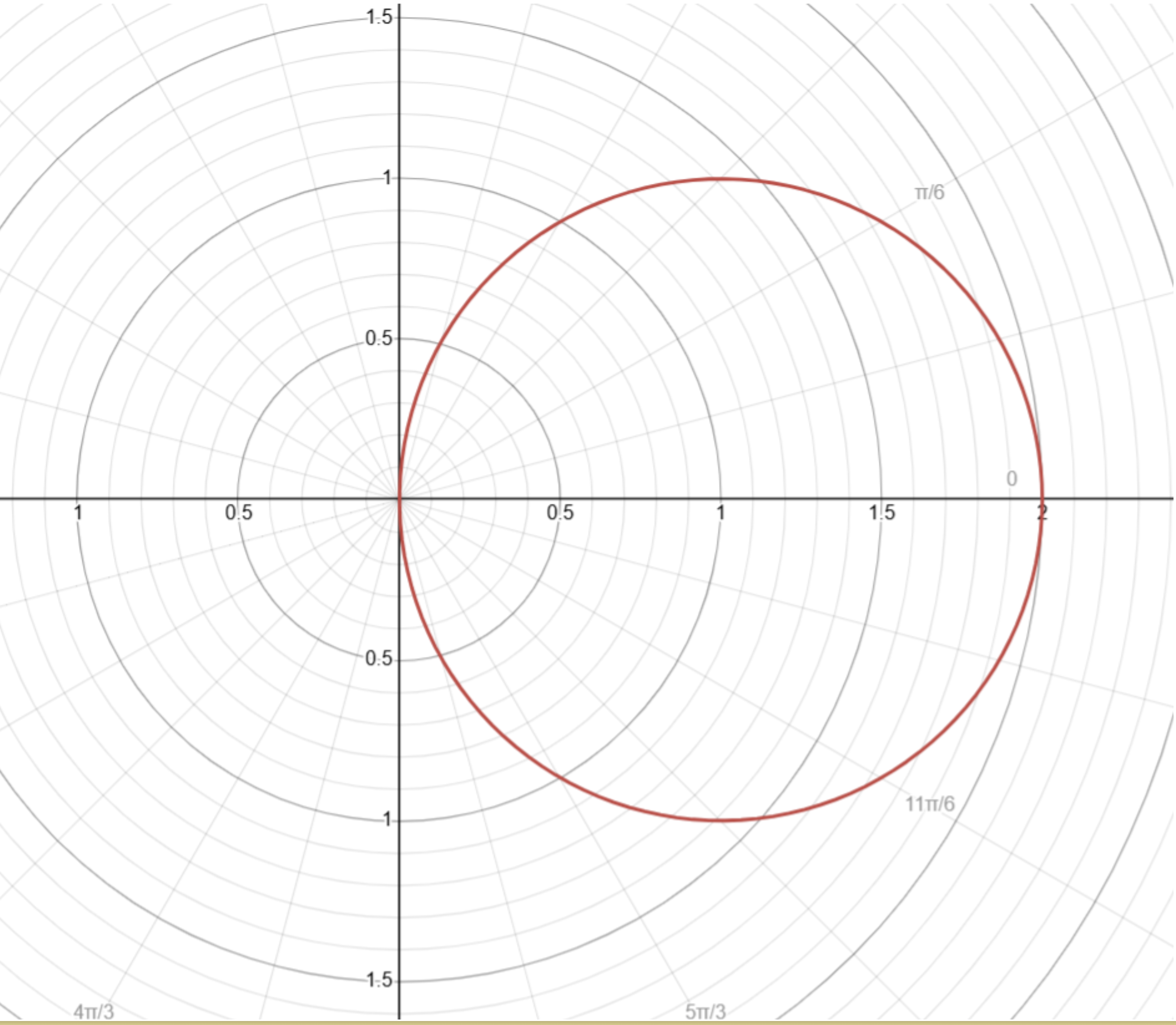
- This is simply a circle of radius on the right side of the graph.
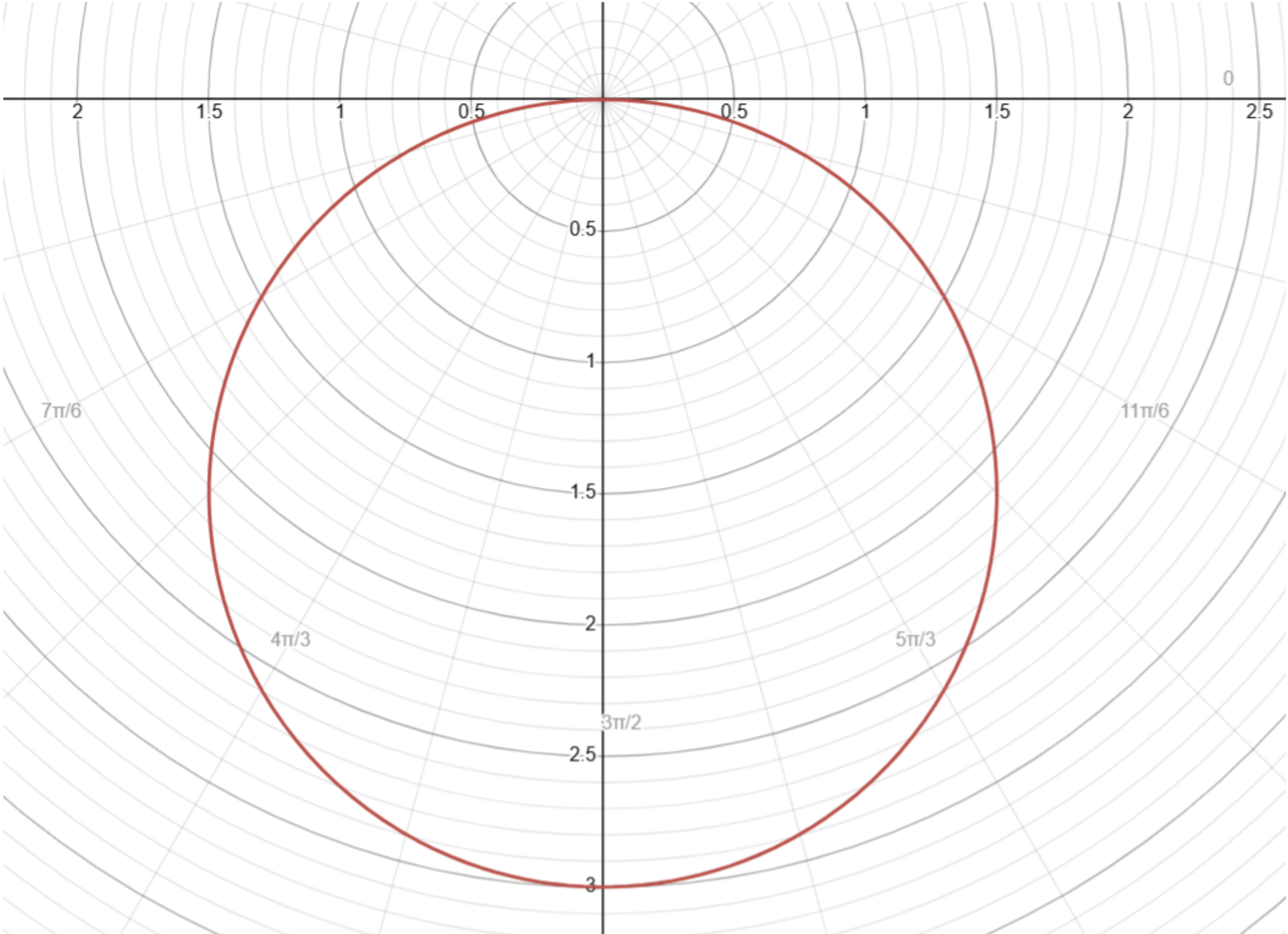
- This is a circle facing down with radius
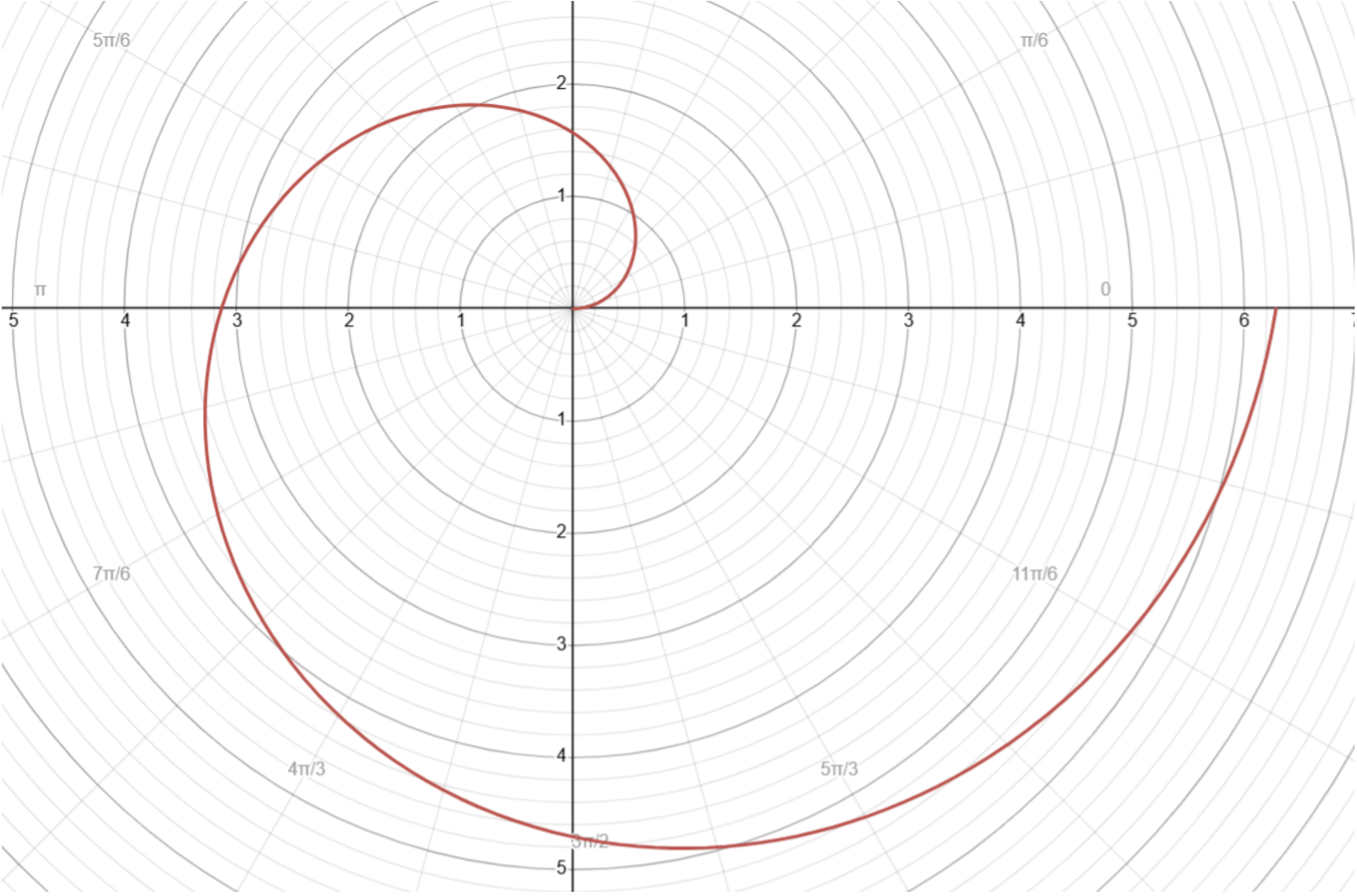
- This is the Archimedean spiral. What value you go to will depend on the size of your graph (typically it is either up to or )
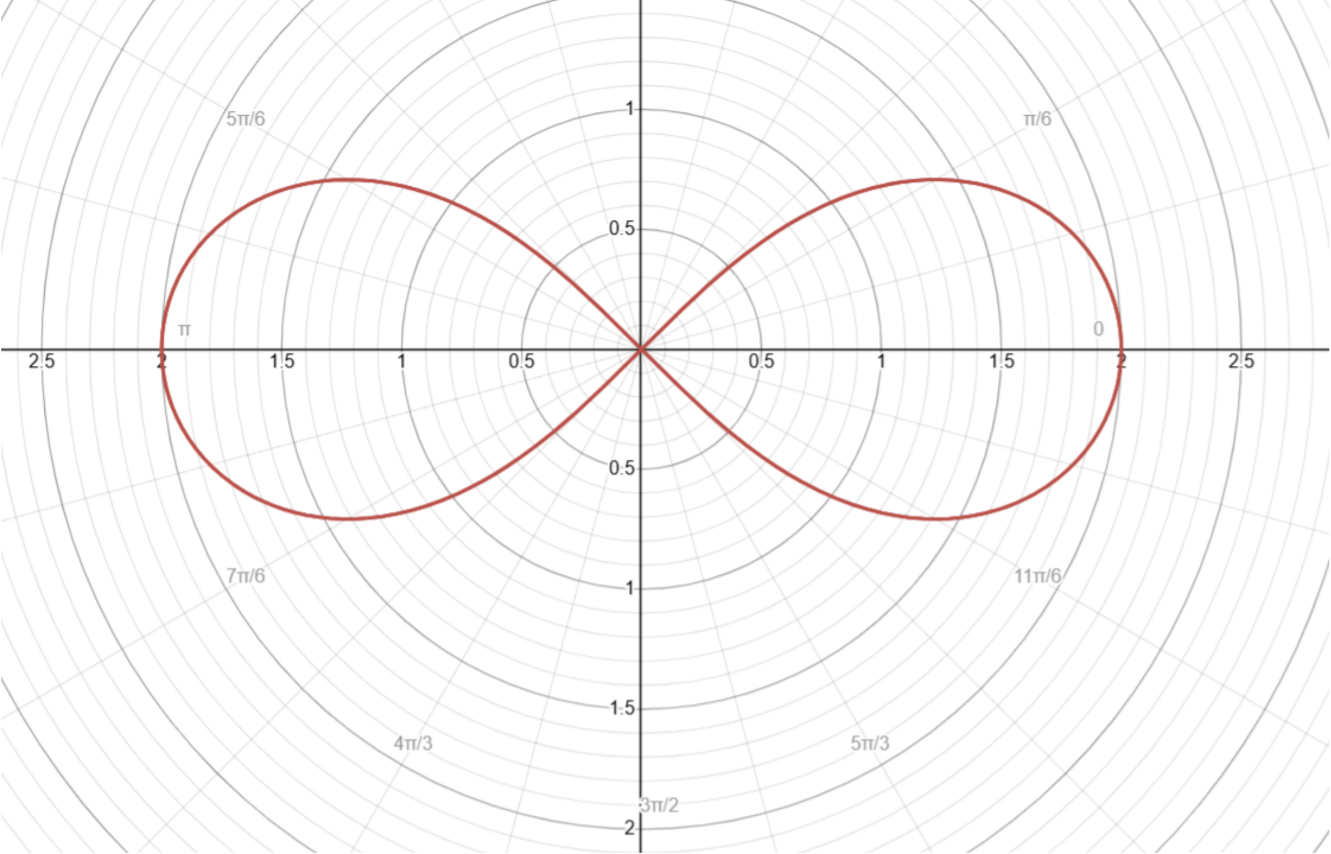
- This is a Lemniscate.
-
-
Use the double-angle identity for sine.
- Now, it is just a lemniscate.
-
Use the double-angle identity for sine.
- This is a cardioid since
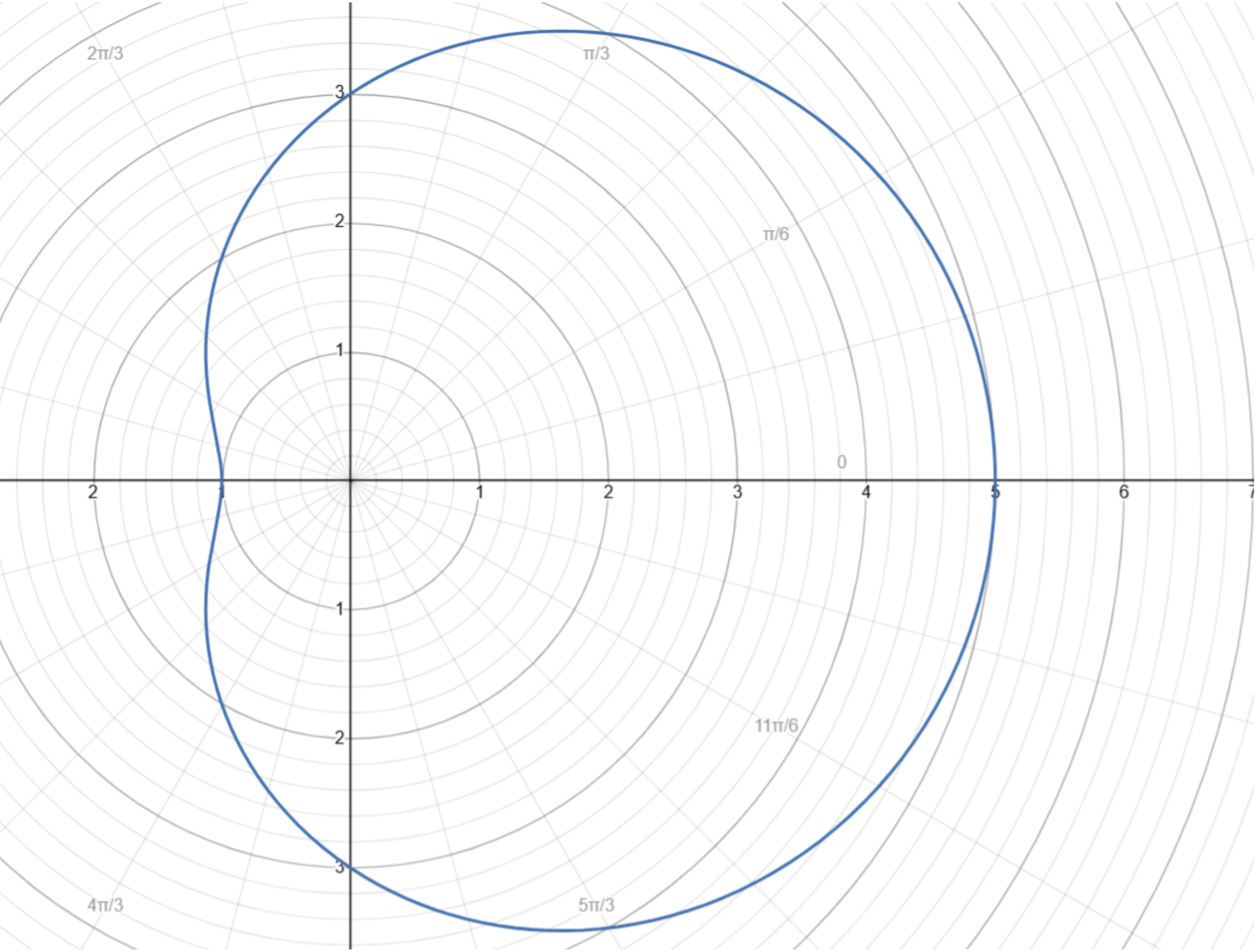
- This is a dimpled limaçon since
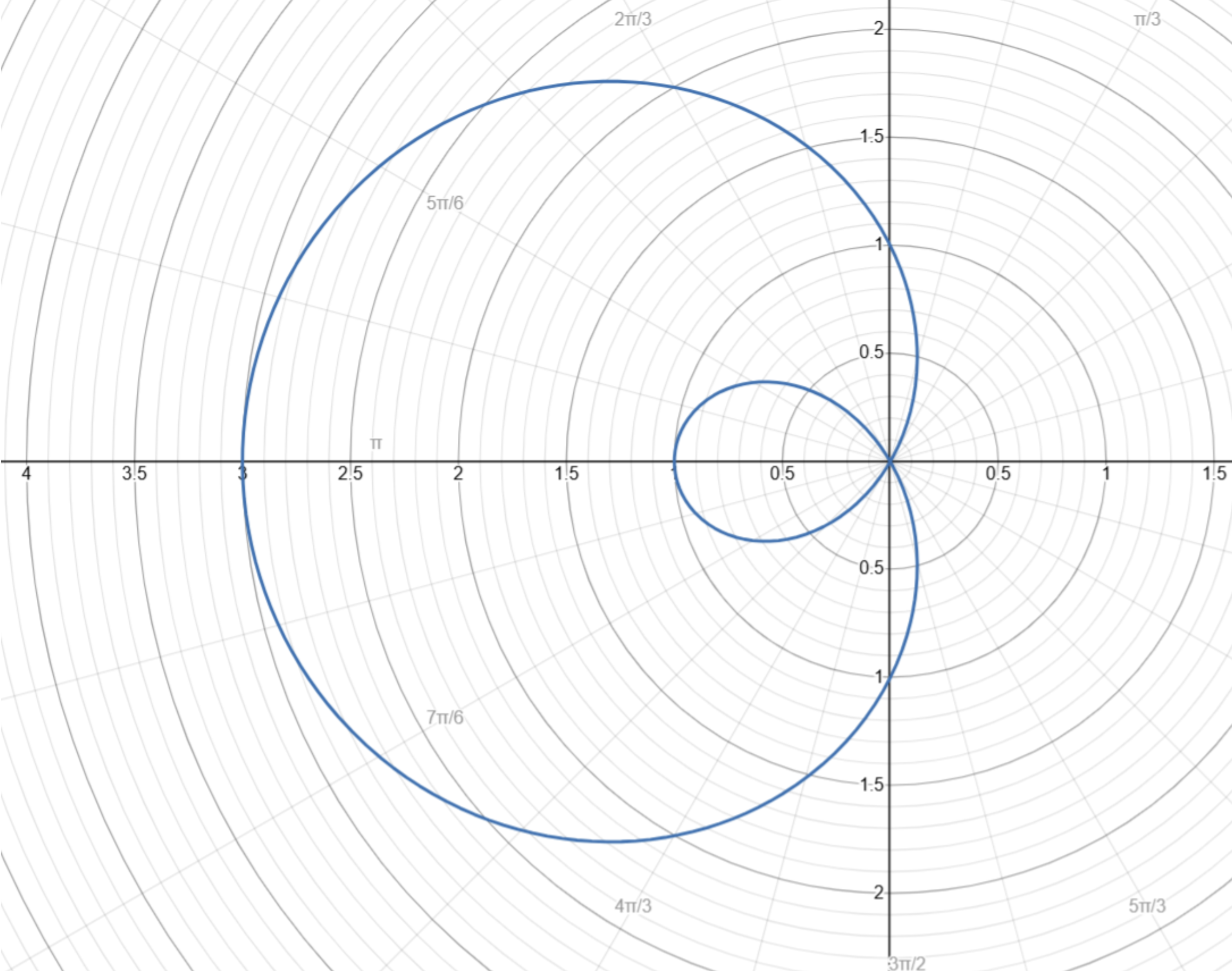
- This is an inner-loop limaçon since
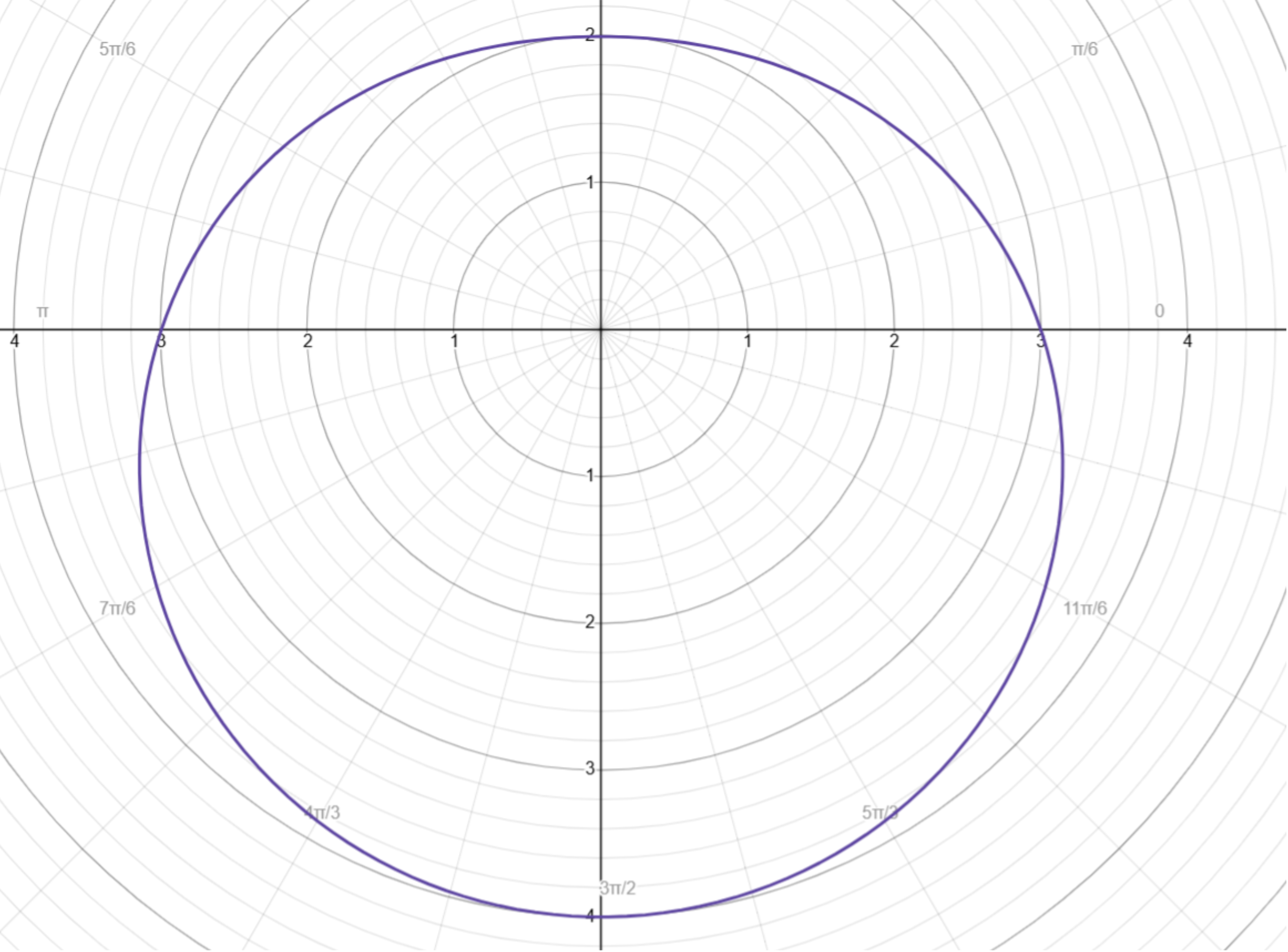
- This is a convex limaçon since
-
-
Once again, we can use the sine double-angle identity
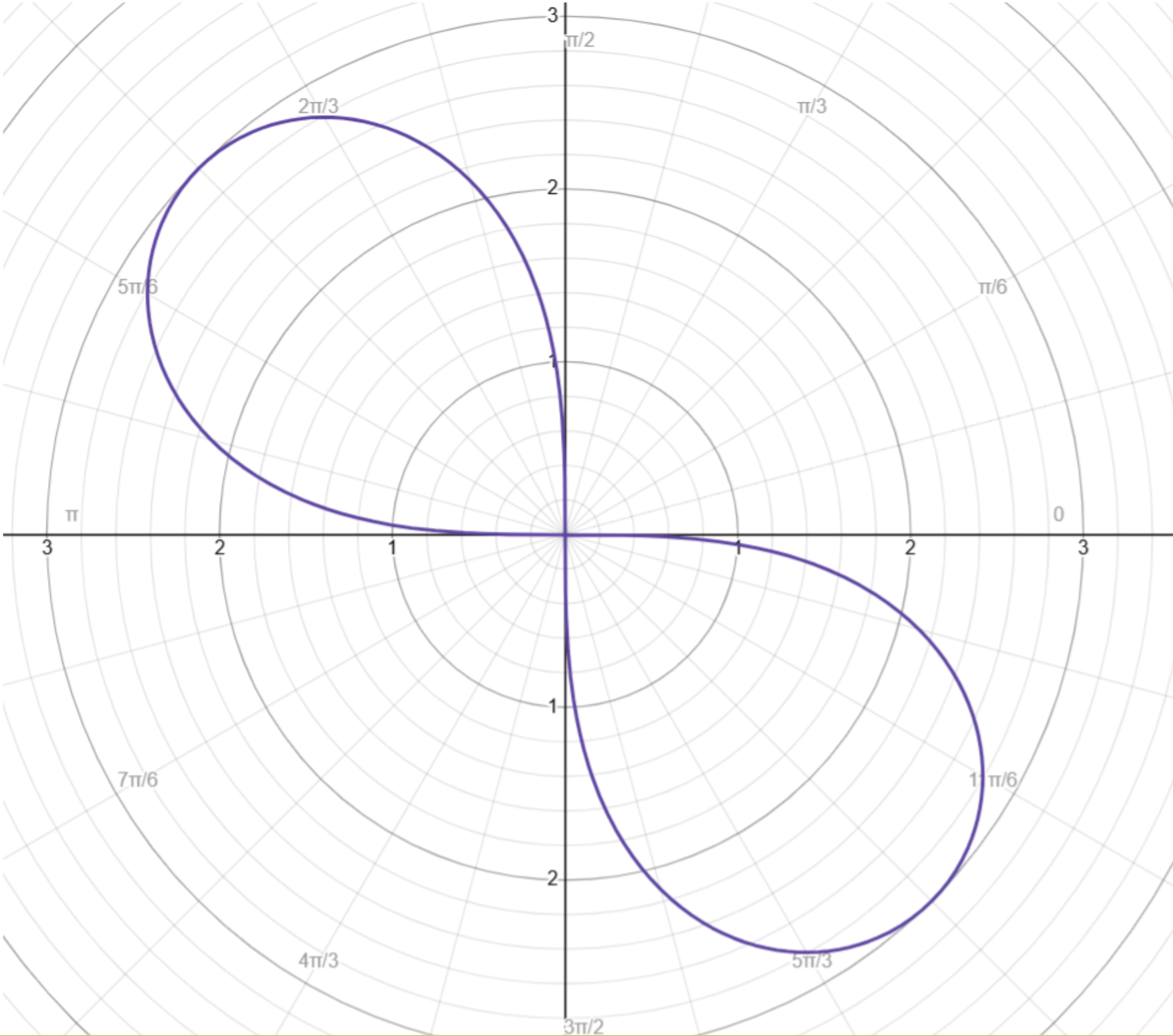
- Thus, it is a lemniscate
-
Once again, we can use the sine double-angle identity
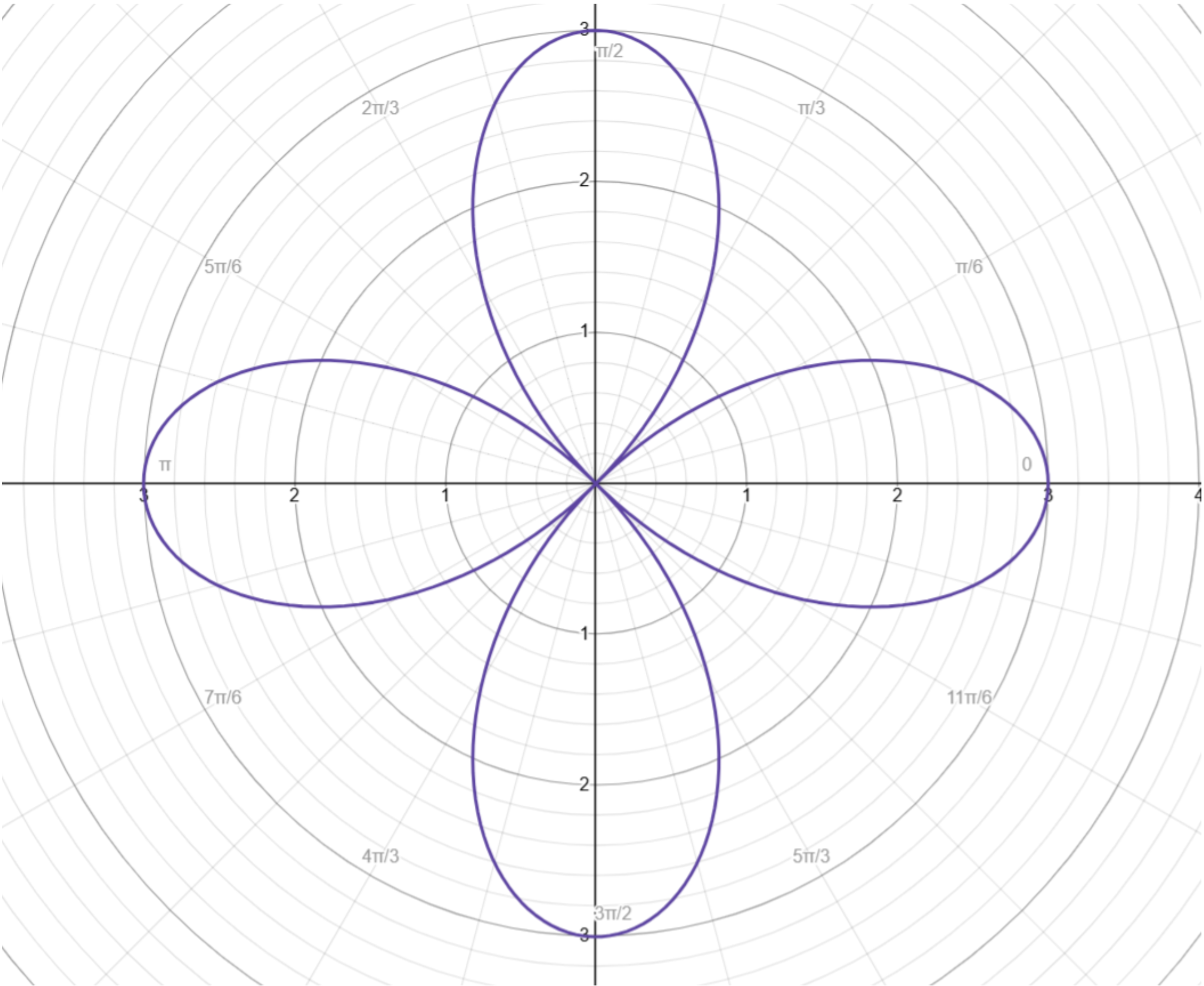
- This is simply a positive cosine rose curve of four petals and max length
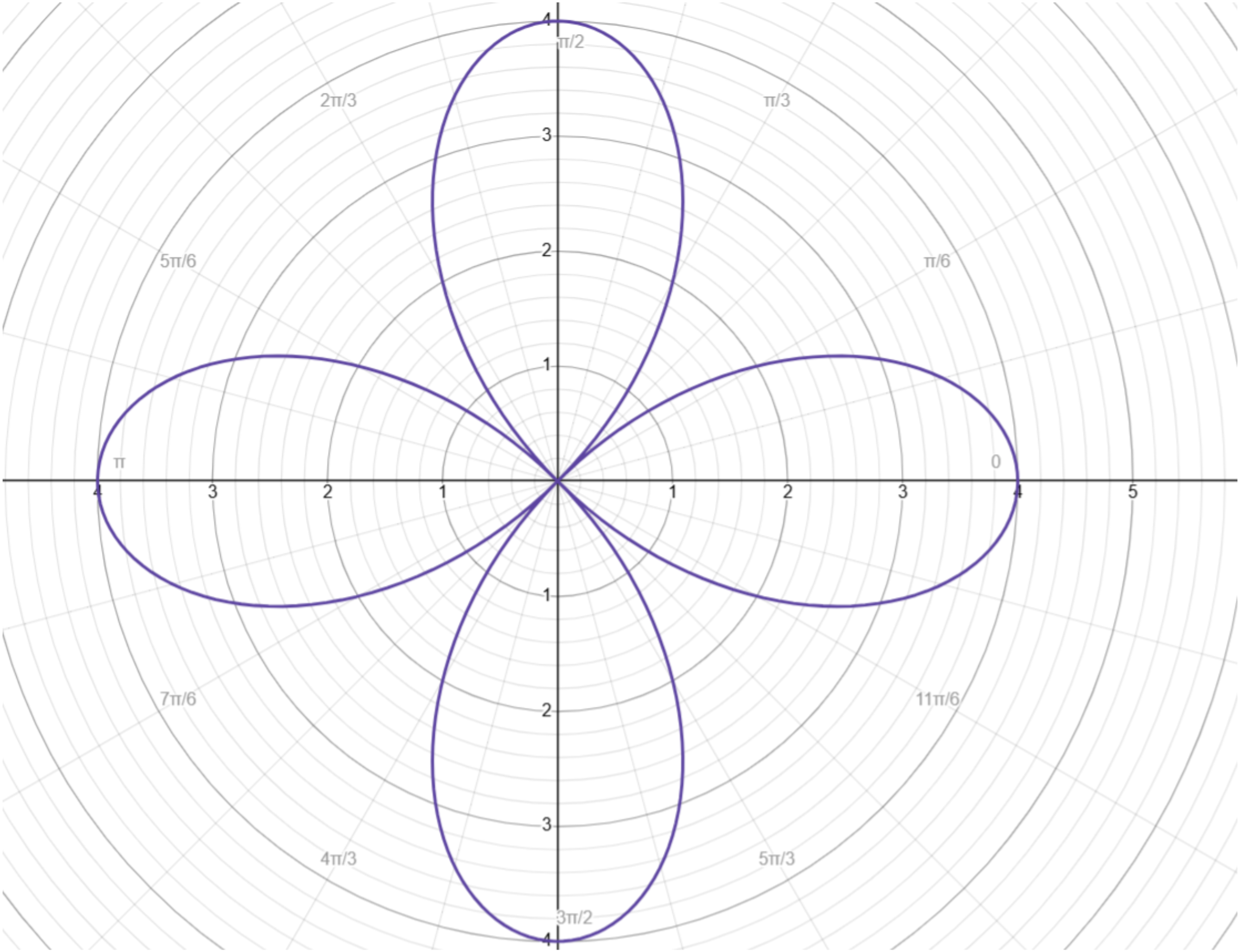
- This is a positive cosine rose curve of four petals and max length
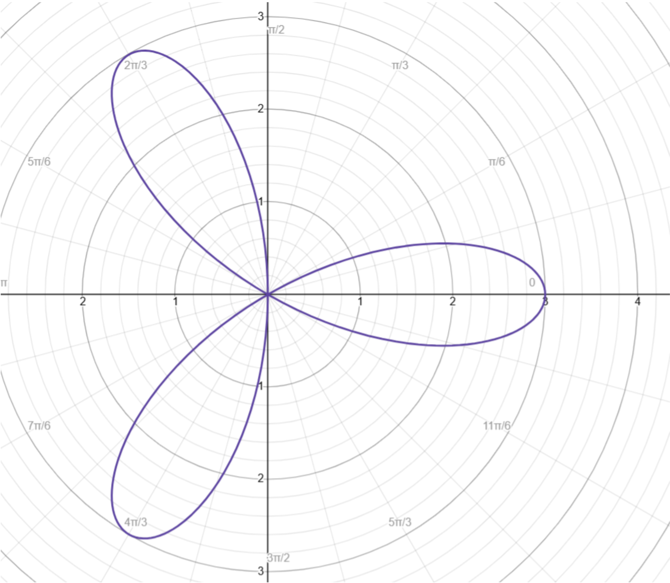
- This is a positive cosine rose curve of petals and max length
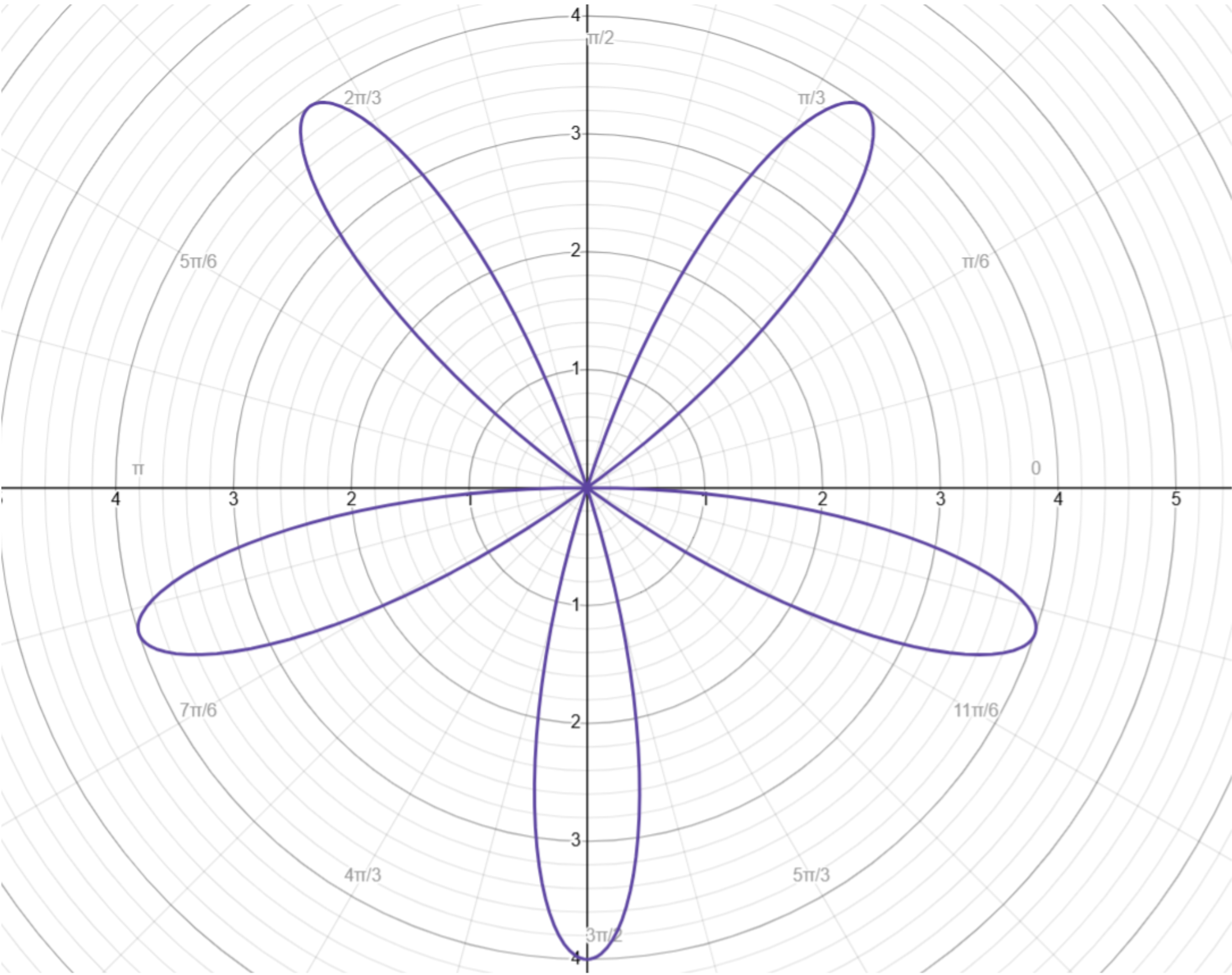
- This is a negative sine rose curve of five petals and max length
- This is a positive sine rose curve of eight petals and max length
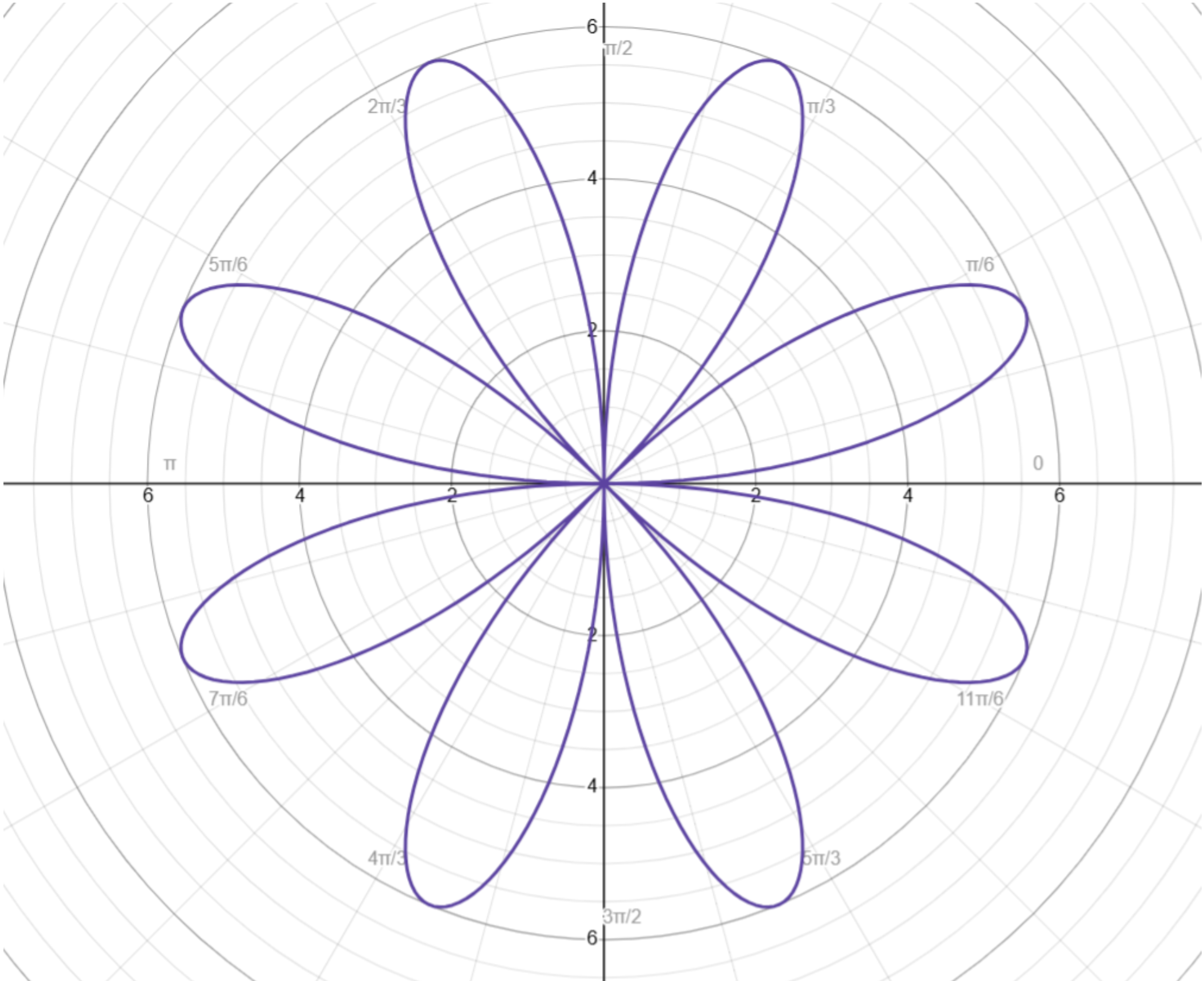
- It is a dimpled limaçon since (and because )
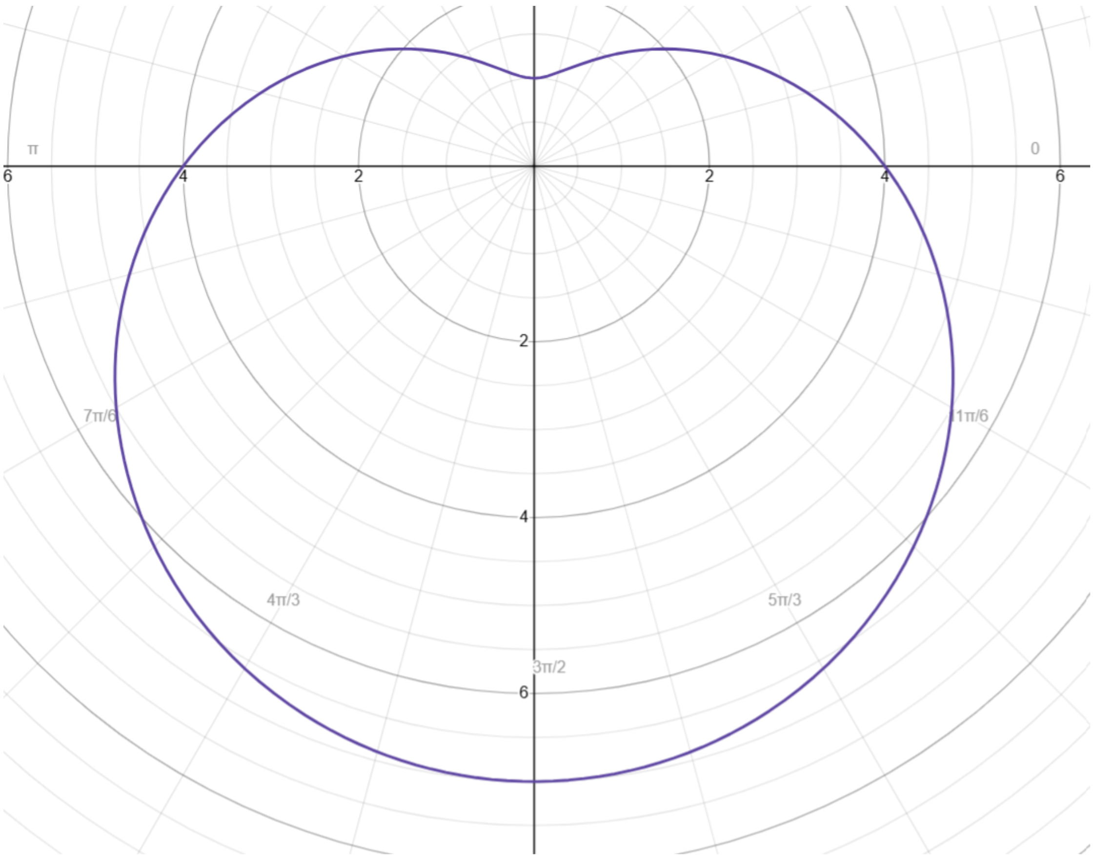
-
- Substituting for and ,
- This is simply a straight-line, or a linear function
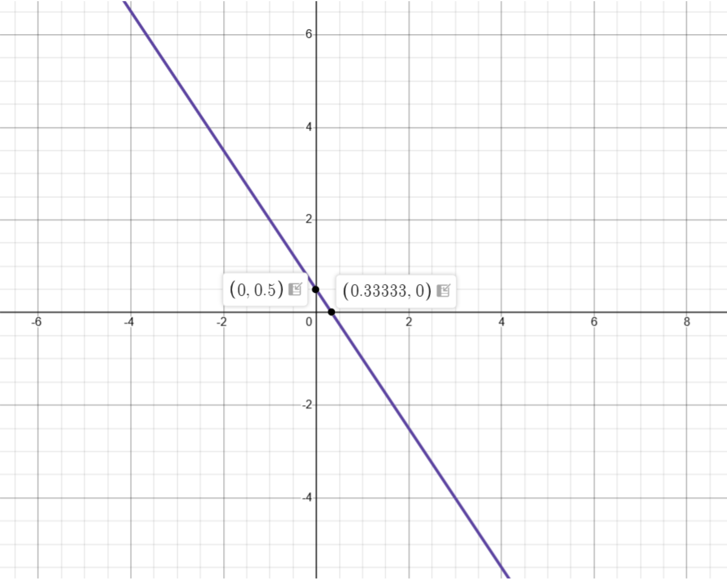
- This is a positive cosine rose curve with eight petals and max length 5
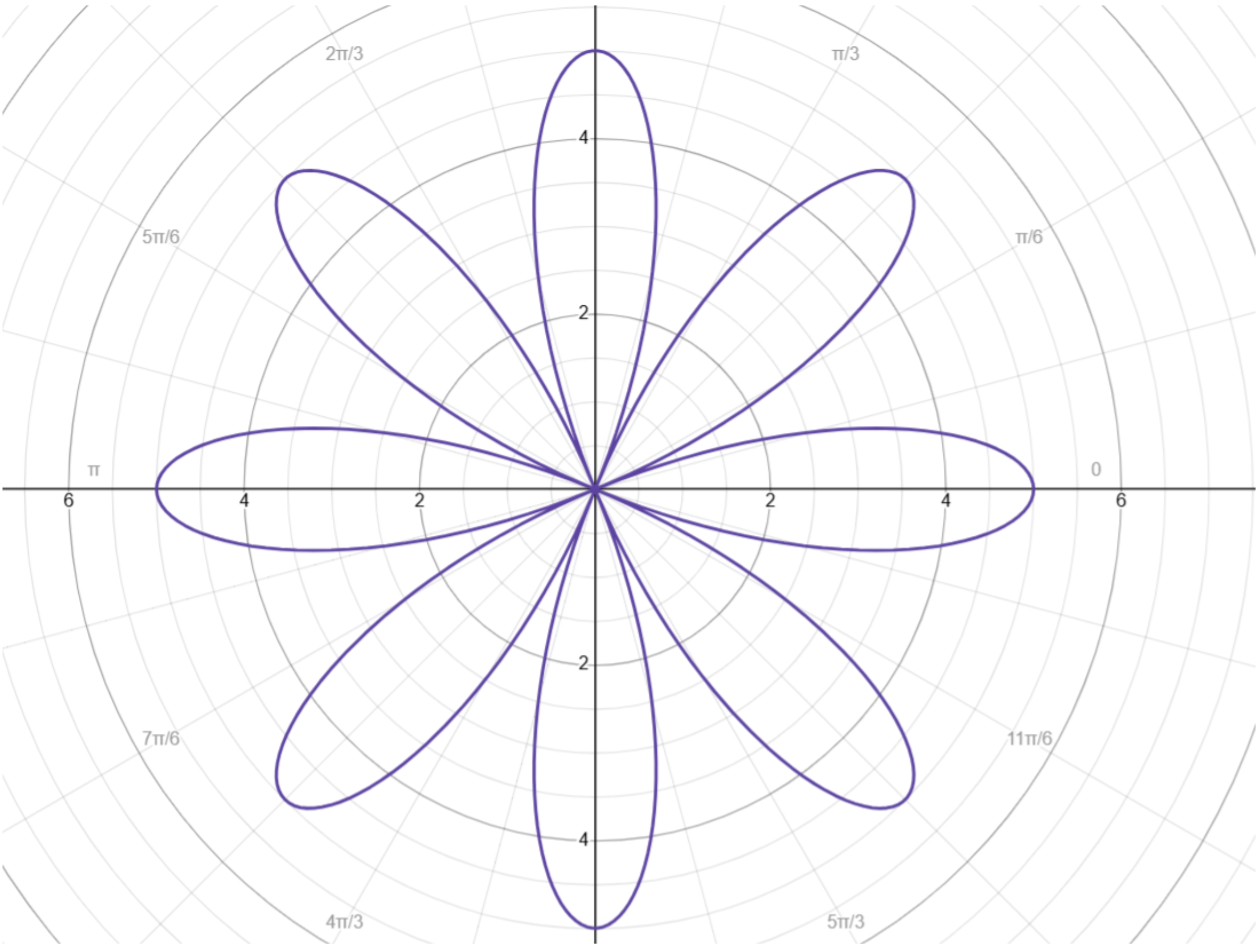
-
-
Substituting ,
-
Let
- Solutions for u are
- Plugging back in,
- On a polar graph, the solution is simply a line (like a linear function but on a polar graph).
- The conversion for is . So,
- Tangent has a period of , so the term only produces two distinct values. When k is even, is
- When k is odd, is
- By the cofunction identity for , we get (used the same method as the first slope)
- Thus, the two solutions are the lines
-
-
Multiply both sides
- Thus, the final form is
- You can leave it like this; typically, you will not have to simplify it further.
-
Multiply both sides
-
This is the formula for a circle centered at with radius 2. Thus, it can be written as .
- These types of problems you can simply imagine.
-
- $@r^{4}=3r\cos\theta
-
Formulas:
-
The max length of the function is 3, meaning . It has 3 petals, meaning
- Typically, it is beneficial to memorize the orientation for cosine and sine depending on whether is positive or negative. Here, when the function lies on the negative polar access, it is a negative cosine function.
- However, you can also find out by testing.
-
Let’s assume is positive:
- The function would be .
- Plugging in , .
- This would be on the positive polar axis. However, for our graph, , meaning .
- So, our answer is
-
Our maximum value is 1, meaning . It has 5 petals, meaning
- When sine has a petal on the “negative y-axis” (note, this doesn’t exist, but it’s simple and most people can tell what it means; it refers to the line ), .
- If you were to test the value of , you should get the same answer, which is .
-
First, we must figure out what function this is. Then, we must figure out how it is graphed. Max value is 2, meaning
- It has 3 petals, meaning .
- Cosine is on the positive polar axis, so . Thus, the function is: .
- To figure out the domain, let’s see how the function is drawn.
- Plugging in , . This is the function’s starting point.
- From here, we can simply move counterclock-wise to see how the function is traced. If you perform this correctly, you will see that half of the first petal (the one that lies on the x-axis) is completed, then it moves onto the petal in the third quadrant, then the 2nd, and finally finishes the first petal last.
- We know that each petal takes the same change of interval to create. Because the total period is , and there are 3 petals, each petal takes up an interval of . Additionally, we know that half a petal takes up an interval of .
-
Thus, the first half of the petal is the interval , and the second half of the petal is the interval .
- But, remember, our interval is , so it repeats on .
- Meaning, our final answer is:
- Or, .
- Though, the first one is clearer.
-
First, let’s figure out the function.
- Max value is 4, meaning . It has 5 petals, meaning Sine is positive when on the positive y-axis, so . Thus, the function is: When , .
- We don’t know where it goes first, so let’s find the next easiest point. When , , meaning it creates the petal that is fully in the first quadrant first (note, we plug in so , which is a known trig value).
- Now, we can simply spin counter clockwise; unlike cosine, sine will not have tricky half-petals made (unless that is the specific interval that you are asked to find). We can see that it’s the second petal drawn. Thus, it begins to be drawn when and ends at . Because the period is only , the complete interval is,
-
As seen by the shape, the function is an inner-loop limaçon.
- Additionally, it faces down, so it must be a negative sine inner-loop limaçon.
- Thus, our basic form is , where and are both positive constants.
- When , the function simply turns to . On the graph, when . Thus, .
- And when , .
- Thus, our formula is
- Now, to find the interval of the inner-loop (the portion highlighted in green), we must find when
- Our interval is , though, so we must find the two other angles.
- The first is (Because sine has same the same value in quadrant 3).
- The second is (because by itself is negative and not within the specified domain)
- Thus, our interval is .