
Introduction
In Topic 4.2, we used parametric functions to describe the position of a particle moving through the plane. We learned how to determine where a particle is, find its horizontal and vertical extrema, and determine when it reaches the coordinate axes.
But just knowing where a particle is does not tell us everything about its motion.
A particle could be moving to the right, to the left, upward, or downward. It could even change direction while following the same path.
So, how can we determine the direction of a particle’s motion?
And how can we measure how quickly its horizontal and vertical position changes?That is what we will be taking a look at in 4.3.
Recall that a parametric function is written as
, ,
where is the parameter.
Analyzing Direction Independently
As we’ve mentioned before, and are two independent functions. This is useful because we can analyze the particle’s horizontal and vertical motion separately.
By looking at whether each function is increasing or decreasing as increases, we can determine the direction of motion of the particle.
Horizontal Direction
Since represents horizontal position:
- If is increasing, the particle is moving to the right.
- If is decreasing, the particle is moving to the left.
Vertical Direction
Since represents vertical position:
- If is increasing, the particle is moving up.
- If is decreasing, the particle is moving down.
Because these two components are independent, their directions can be combined. For example, if is increasing while is decreasing, the particle is moving down and to the right.
The direction can also change as changes. A particle might be moving right and up at , then left and up at . This allows a parametric function to describe complicated paths, including curves that change direction and loops!
Determining Direction from a Table
One of the easiest ways to determine direction is by looking at a table of values.
Suppose we have the following parametric function:
and
.
Consider the following values
As increases, increases.
Therefore, the particle is moving to the right.
At the same time, also increases, so the particle is moving upward.
Therefore, over this interval, the particle is moving up and to the right.
Being able to analyze the horizontal and vertical components independently is incredibly important, as the particle’s overall direction is determined by combining those two pieces of information.
Combining Horizontal and Vertical Motion
There are four basic combinations of horizontal and vertical motion.
If is increasing and is increasing, the particle moves up and right.
If is decreasing and is increasing, the particle moves up and left.
If is decreasing and is decreasing, the particle moves down and left.
If is increasing and is decreasing, the particle moves down and right.
We can summarize this with a table:
Example
Suppose
and
.
What direction is the particle moving at ?
As increases, the value of decreases. Therefore, the particle is moving to the left.
Now, we examine .
As increases around , the value of increases. Therefore, the particle is moving upward.
Combining these two pieces of information, we find that the particle is moving up and to the left.
Let’s look at another example.
Suppose
and
.
What direction is the particle moving at ?
Again, we look at .
As increases, the value of increases. Therefore, the particle is moving to the right.
And looking at , we see that as increases, the value of decreases. Therefore, the particle is moving downward.
Combining what we found, we now know the particle is moving down and to the right.
Direction Can Change
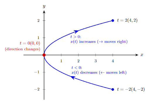
A particle does not necessarily travel in the same direction throughout its entire motion.
For example, consider
and
.
For negative values of , as increases towards 0, decreases.
Therefore, the particle moves to the left.
After , begins increasing, so the particle moves to the right, changing direction.
The Same Point Can Have Different Directions
Here’s where parametric motion becomes particularly interesting.
A particle can pass through the same point more than once, and it does not necessarily have to travel in the same direction each time.
Imagine a particle traveling around a loop.
Eventually, it may return to a point it has already visited.
The particle could pass through that point while moving upward the first time and then pass through it later while moving downward.
The coordinates of the point are identical, but the particle’s direction is different.
Therefore, only knowing the point does not necessarily tell us the direction of motion; we also need to know the parameter value .
According to the AP Precalculus Course and Exam Description (p.118):
“At any given point in the plane, the direction of planar motion may be different for different values of .”
The parameter is therefore doing more than simply identifying a point. It tells us where the particle is along its motion through the curve.
Different Parametrizations of the Same Curve
There is another important consequence of this idea: the same curve can have multiple parametric representations.
Consider the circle
.
One possible parametrization is
As increases from 0 to , the particle travels around the circle.
But we could instead write
Using the identities
and
,
this becomes
,
This still traces the same circle, but the particle travels around it in the opposite direction.
So, two parametric functions can describe the same geometric curve while producing different motion along that curve.
Key Takeaways:
The curve tells us where the particle can go.
The parametrization tells us how the particle moves along the curve.
Traversing a Curve in Different Directions
Let’s make this idea even simpler.
Imagine walking around a circular track. The track itself does not change depending on whether you walk clockwise or counterclockwise; the path itself is the same, but the direction of travel is different.
Parametric functions work the same way. Two different parametrizations can describe the same curve while causing the particle to traverse that curve in different directions. This means that when analyzing a parametric function, we should distinguish between the shape of the path and the direction in which the path is traversed.
This is one of the major differences between a parametric representation and an ordinary equation such as . A rectangular equation primarily describes the geometric relationship between and , while a parametric equation can describe that relationship and how a particle moves through it.
Average Rate of Change
So far, we have talked about whether and are increasing or decreasing. Now, we can ask a more quantitative question:
How quickly are they changing?
To answer this, we need to take a look aaallllll the way back into Unit 1.2: Rates of Change!
Recall that for an ordinary function , the average rate of change from to $@x=b is
.
The same basic idea applies to each component of a parametric function.
For
,
the average rate of change of horizontal position from to is
.
Similarly, for
the average rate of change of vertical position is
.
As you may have guessed, these two qualities can also be analyzed independently.
Average Rate of Change in Both Directions
Now, let’s combine the two.
Suppose
and
We want to analyze the particle from to .
For the horizontal position,
, .
Therefore,
For the vertical position,
,
Therefore,
.
So, over this interval,
, and .
This means that the particle moves right and upward on average.
But, we can extract even more information from these two rates.
The Slope of a Parametric Curve
Recall that the slope of a line is .
We can rewrite this using the parameter.
Since and both occur over the same change in , we can write
Therefore, for two points on a parametric curve:
provided that
.
More explicitly:
.
The factors of cancel, leaving
So this is simply the familiar slope formula applied to the two points generated by the parameter values.
Example
Suppose , and .
Find the slope of the line connecting the points corresponding to and .
We can see that and .
Therefore, the slope is
Thus,
We can also obtain the same result from the average rates of change.
The average vertical rate is
and the average horizontal rate is
Therefore,
.